Chapter 9 Peak Normalization
9.1 Batch effects
Batch effects are sources of variation that arise from factors other than the biological design of the study. A simple model for the intensity of one peak is:
\[Intensity = Average + Condition + Batch + Error\]
The main scientific interest is usually the condition term, while the average and random error can often be estimated directly. The batch contribution is more difficult, because some technical drivers are known, such as injection order or operator, but many are only partially observed or completely hidden. Most batch-correction methods attempt to estimate and remove this unwanted variation without erasing the biological signal of interest.
In analytical chemistry, internal standards or pooled quality-control samples often serve as proxies for the batch term in this model. However, it is impractical to cover the entire metabolome with internal standards in untargeted data. In methods based on internal standards or pooled QC samples, variation is usually adjusted by median, quantile, mean, or ratio-based correction. Other approaches, such as quantile regression, centering, and scaling based on within-sample intensity distributions, similarly rely on stable signal structure to reduce batch effects.
9.2 Batch effects classification
Variances among the samples across all the extracted peaks might be affected by factors other than the experiment design. There are three types of those batch effects: Monotone, Block and Mixed.
- Monotone would increase/decrease with the injection order or batches.
- Block would be system shift among different batches.
- Mixed would be the combination of monotone and block batch effects.

Meanwhile, different compounds would suffer different type of batch effects. In this case, the normalization or batch correction should be done peak by peak.
9.3 Batch effects visualization
Any correction might introduce bias. We need to make sure there are patterns which different from our experimental design. Pooled QC samples should be clustered on PCA score plot.
9.4 Source of batch effects
Different Operators & Dates & Sequences
Different Instrumental Condition such as different instrumental parameters, poor quality control, sample contamination during the analysis, Column (Pooled QC) and sample matrix effects (ions suppression or/and enhancement)
Unknown Unknowns
9.5 Avoid batch effects by DoE
You could avoid batch effects from experimental design. Cap the sequence with Pooled QC and Randomized samples sequence. Some internal standards/Instrumental QC might Help to find the source of batch effects while it’s not practical for every compounds in non-targeted analysis.
Batch effects might not change the conclusion when the effect size is relatively small. Here is a simulation:
set.seed(30)
# real peaks
group <- factor(c(rep(1,5),rep(2,5)))
con <- c(rnorm(5,5),rnorm(5,8))
re <- t.test(con~group)
# real peaks
group <- factor(c(rep(1,5),rep(2,5)))
con <- c(rnorm(5,5),rnorm(5,8))
batch <- seq(0,5,length.out = 10)
ins <- batch+con
re <- t.test(ins~group)

index <- sample(10)
ins <- batch+con[index]
re <- t.test(ins~group[index])
Randomization could not guarantee the results. Here is a simulation.
9.6 post hoc data normalization
To make the samples comparable, normalization across the samples are always needed when the experiment part is done. Batch effect should have patterns other than experimental design, otherwise just noise. Correction is possible by data analysis/randomized experimental design. There are numerous methods to make normalization with their combination. We could divided those methods into two categories: unsupervised and supervised.
Unsupervised methods only consider the normalization peaks intensity distribution across the samples. For example, quantile calibration try to make the intensity distribution among the samples similar. Such methods are preferred to explore the inner structures of the samples. Internal standards or pool QC samples also belong to this category. However, it’s hard to take a few peaks standing for all peaks extracted.
Supervised methods will use the group information or batch information in experimental design to normalize the data. A linear model is always used to model the unwanted variances and remove them for further analysis.
Since the real batch effects are always unknown, it’s hard to make validation for different normalization methods. Li et al. developed NOREVA to make comparison among 25 correction method (B. Li et al. 2017) and a recently updates make this numbers to 168 (Yang et al. 2020). MetaboDrift also contain some methods for batch correction in excel (Thonusin et al. 2017). Another idea is use spiked-in samples to validate the methods (Franceschi et al. 2012) , which might be good for targeted analysis instead of non-targeted analysis.
Relative log abundance (RLA) plots(De Livera et al. 2012) and heatmap often used to show the variances among the samples.
9.7 Method selection flowchart
In practice, the choice of normalization method should begin with study design rather than with software availability.
Are pooled QC samples available across the analytical run?
If yes, QC-based methods such as ratio normalization, regression-based correction, SERRF, or QC-aware drift models are often strong first choices.Are stable isotope-labeled internal standards available for the compounds or classes of interest?
If yes, internal-standard-based correction should usually be prioritized for those targets.Is the batch structure known?
If yes, supervised methods such as ComBat, regression calibration, or other model-based approaches can be considered.Is the major problem global scale difference or feature-specific drift?
Global scale differences may respond to centering, scaling, or total-abundance normalization, while feature-specific drift usually needs peak-wise correction.Is the study exploratory or confirmatory?
Exploratory studies often prefer more conservative methods that do not overfit. Confirmatory or large-cohort studies may justify more complex supervised correction.
As a rough guide:
Have pooled QC and obvious drift: start with QC-based correction or SERRF.
Have known batch labels but limited QC: consider regression-based methods or ComBat, while checking group-batch confounding carefully.
Have strong internal standards for a targeted panel: internal-standard normalization should be primary.
Have no QC and no reliable batch covariates: use conservative unsupervised normalization and interpret results cautiously.
Have strong hidden unwanted variation: consider latent factor methods such as SVA, RUV, or RRmix.
9.7.1 Unsupervised methods
9.7.1.1 Distribution of intensity
Intensity collects from LC/GC-MS always showed a right-skewed distribution. Log transformation is often necessary for further statistical analysis.
9.7.1.2 Centering
For peak p of sample s in batch b, the corrected abundance I is:
\[\hat I_{p,s,b} = I_{p,s,b} - mean(I_{p,b}) + median(I_{p,qc})\]
If no quality control samples used, the corrected abundance I would be:
\[\hat I_{p,s,b} = I_{p,s,b} - mean(I_{p,b})\]
9.7.1.3 Scaling
For peak p of sample s in certain batch b, the corrected abundance I is:
\[\hat I_{p,s,b} = \frac{I_{p,s,b} - mean(I_{p,b})}{std_{p,b}} * std_{p,qc,b} + mean(I_{p,qc,b})\] If no quality control samples used, the corrected abundance I would be:
\[\hat I_{p,s,b} = \frac{I_{p,s,b} - mean(I_{p,b})}{std_{p,b}}\]
9.7.1.4 Pareto Scaling
For peak p of sample s in certain batch b, the corrected abundance I is:
\[\hat I_{p,s,b} = \frac{I_{p,s,b} - mean(I_{p,b})}{Sqrt(std_{p,b})} * Sqrt(std_{p,qc,b}) + mean(I_{p,qc,b})\]
If no quality control samples used, the corrected abundance I would be:
\[\hat I_{p,s,b} = \frac{I_{p,s,b} - mean(I_{p,b})}{Sqrt(std_{p,b})}\]
9.7.1.5 Range Scaling
For peak p of sample s in certain batch b, the corrected abundance I is:
\[\hat I_{p,s,b} = \frac{I_{p,s,b} - mean(I_{p,b})}{max(I_{p,b}) - min(I_{p,b})} * (max(I_{p,qc,b}) - min(I_{p,qc,b})) + mean(I_{p,qc,b})\]
If no quality control samples used, the corrected abundance I would be:
\[\hat I_{p,s,b} = \frac{I_{p,s,b} - mean(I_{p,b})}{max(I_{p,b}) - min(I_{p,b})} \]
9.7.1.6 Level scaling
For peak p of sample s in certain batch b, the corrected abundance I is:
\[\hat I_{p,s,b} = \frac{I_{p,s,b} - mean(I_{p,b})}{mean(I_{p,b})} * mean(I_{p,qc,b}) + mean(I_{p,qc,b})\]
If no quality control samples used, the corrected abundance I would be:
\[\hat I_{p,s,b} = \frac{I_{p,s,b} - mean(I_{p,b})}{mean(I_{p,b})} \]
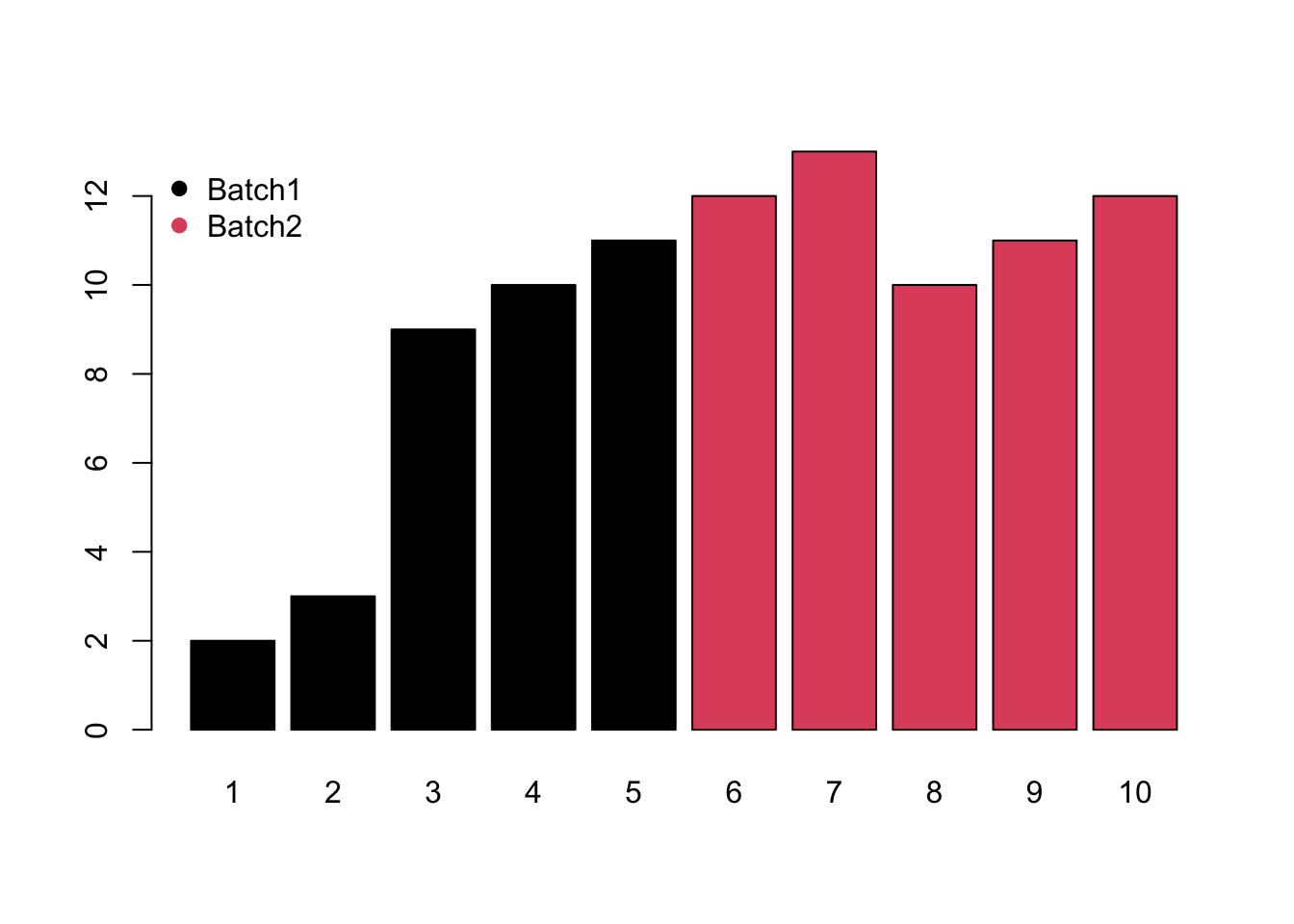
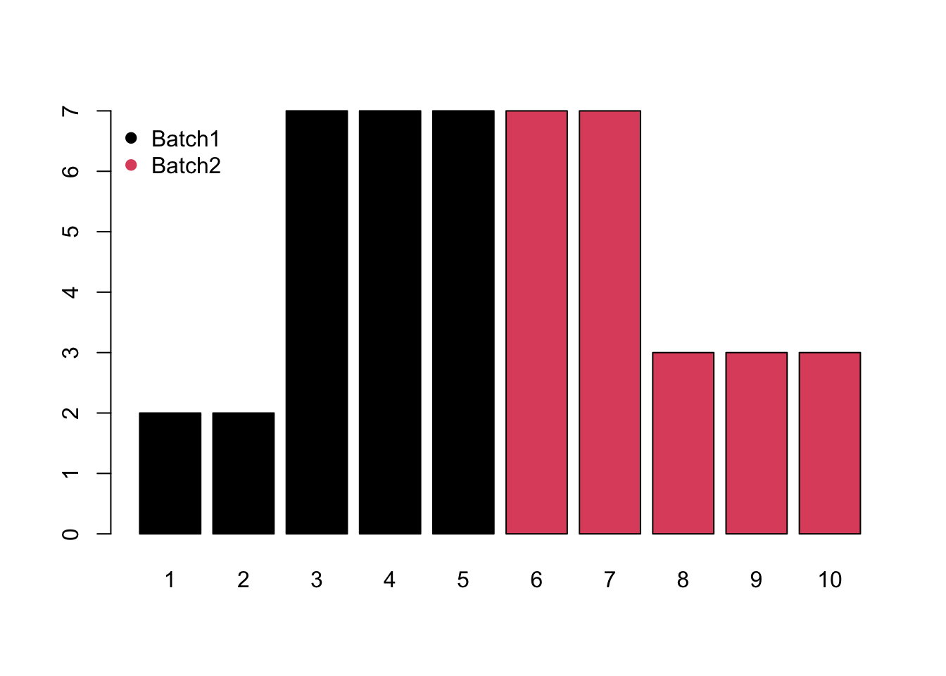
9.7.1.7 Quantile
The idea of quantile calibration is that alignment of the intensities in certain samples according to quantile in each sample.
Here is the demo:
set.seed(42)
a <- rnorm(1000)
# b sufferred batch effect with a bias of 10
b <- rnorm(1000,10)
hist(a,xlim=c(-5,15),breaks = 50)
hist(b,col = 'black', breaks = 50, add=T)
# quantile normalized
cor <- (a[order(a)]+b[order(b)])/2
# reorder
cor <- cor[order(order(a))]
hist(cor,col = 'red', breaks = 50, add=T)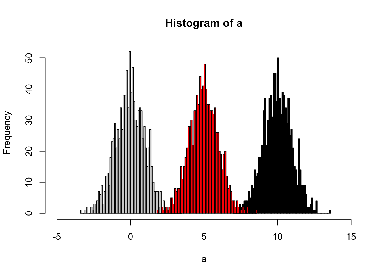
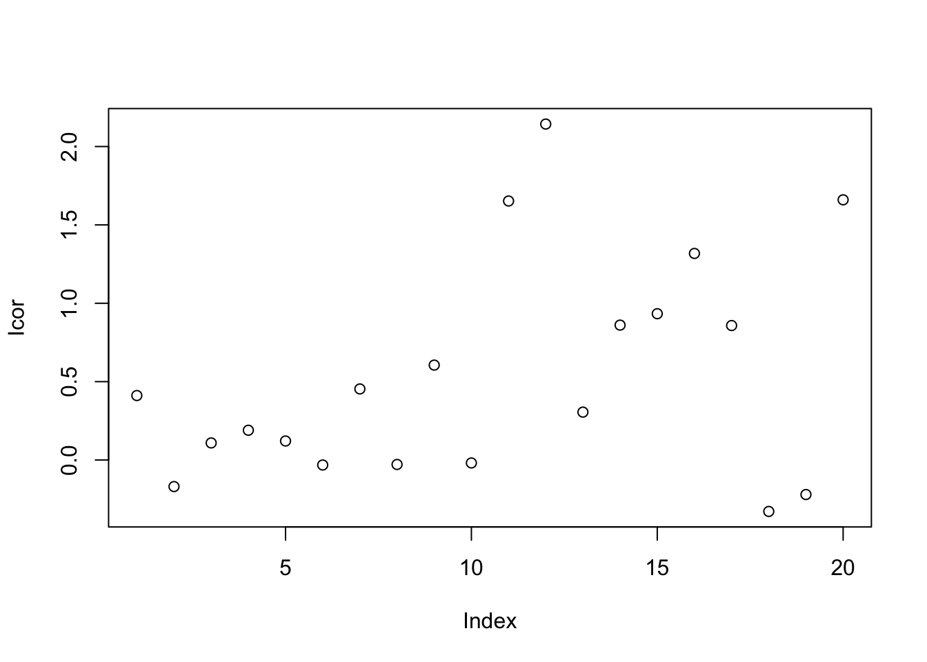
9.7.1.8 Ratio based calibration
This method calibrates samples by the ratio between qc samples in all samples and in certain batch.For peak p of sample s in certain batch b, the corrected abundance I is:
\[\hat I_{p,s,b} = \frac{I_{p,s,b} * median(I_{p,qc})}{mean_{p,qc,b}}\]
set.seed(42)
# raw data
I = c(rnorm(10,mean = 0, sd = 0.3),rnorm(10,mean = 1, sd = 0.5))
# batch
B = c(rep(0,10),rep(1,10))
# qc
Iqc = c(rnorm(1,mean = 0, sd = 0.3),rnorm(1,mean = 1, sd = 0.5))
# corrected data
Icor = I * median(c(rep(Iqc[1],10),rep(Iqc[2],10)))/mean(c(rep(Iqc[1],10),rep(Iqc[2],10)))
# plot the result
plot(I)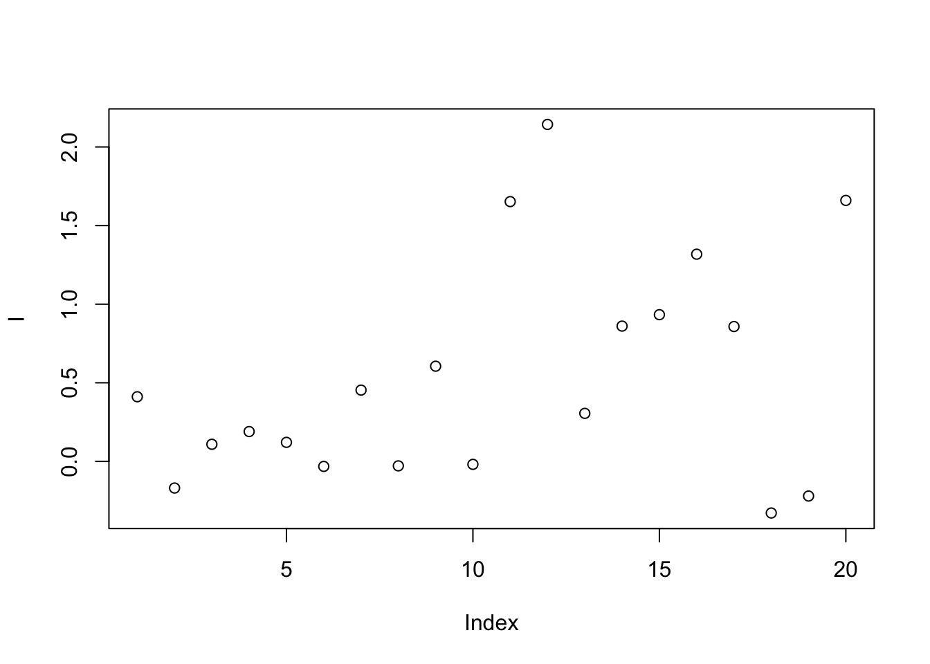
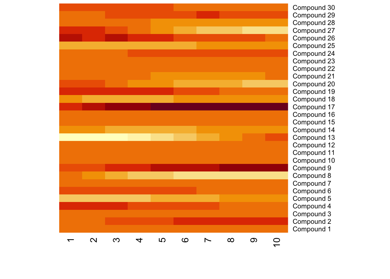
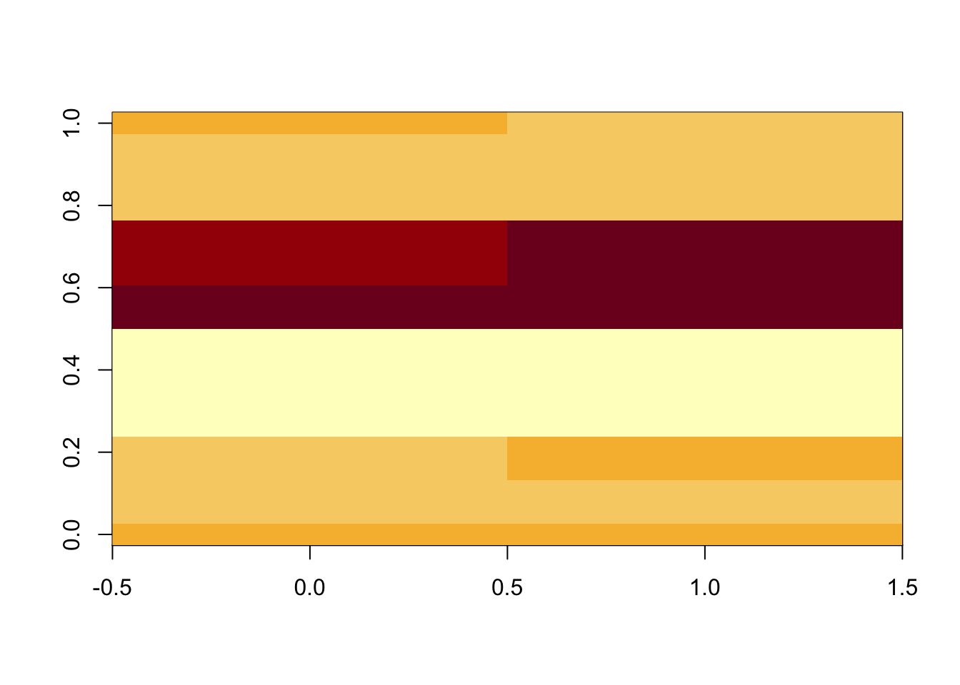
9.7.1.9 Linear Normalizer
This method initially scales each sample so that the sum of all peak abundances equals one. In this study, by multiplying the median sum of all peak abundances across all samples,we got the corrected data.
set.seed(42)
# raw data
peaksa <- c(rnorm(10,mean = 10, sd = 0.3),rnorm(10,mean = 20, sd = 0.5))
peaksb <- c(rnorm(10,mean = 10, sd = 0.3),rnorm(10,mean = 20, sd = 0.5))

df <- rbind(peaksa,peaksb)
dfcor <- df/apply(df,2,sum)* sum(apply(df,2,median))

image(df)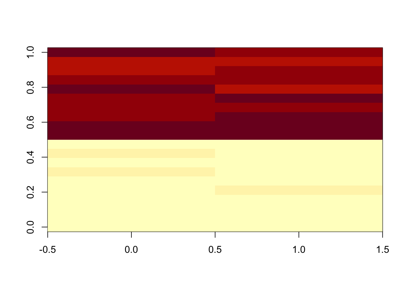
9.7.1.10 Internal standards
\[\hat I_{p,s} = \frac{I_{p,s} * median(I_{IS})}{I_{IS,s}}\]
Some methods also use pooled calibration samples and multiple internal standard strategy to correct the data (van der Kloet et al. 2009; Sysi-Aho et al. 2007). Also some methods only use QC samples to handle the data (Kuligowski et al. 2015).
9.7.1.11 Practical R examples
The following toy examples illustrate common normalization ideas in R.
Log transformation and autoscaling
set.seed(1)
x <- matrix(rexp(50, rate = 0.2), nrow = 10)
x_log <- log2(x + 1)
x_scaled <- scale(x_log)
head(x_scaled)
## [,1] [,2] [,3] [,4] [,5]
## [1,] 0.2165556 0.36510318 1.20394746 1.3176471 0.2693027
## [2,] 0.7207914 -0.48094713 -0.07556624 -1.6931835 0.1752735
## [3,] -1.1717488 0.19482061 -0.68768185 -0.4573974 0.6198642
## [4,] -1.1953094 2.16022513 -0.18428665 1.2041016 0.5591485
## [5,] -0.3388630 -0.03432190 -1.23786319 -0.8649632 -0.9369751
## [6,] 1.8224954 -0.06040298 -1.42774478 0.8641858 -1.8710526Internal-standard-based correction
set.seed(2)
feature <- rnorm(10, 1000, 150)
is_signal <- rnorm(10, 500, 40)
feature_cor <- feature * median(is_signal) / is_signal
cbind(feature, feature_cor)
## feature feature_cor
## [1,] 865.4628 865.9524
## [2,] 1027.7274 985.2824
## [3,] 1238.1768 1321.7957
## [4,] 830.4436 936.5741
## [5,] 987.9622 894.0741
## [6,] 1019.8630 1293.7262
## [7,] 1106.1932 1068.6840
## [8,] 964.0453 993.9723
## [9,] 1297.6711 1241.2164
## [10,] 979.1819 978.6287Simple QC-based drift correction by injection order
set.seed(3)
inj <- 1:12
qc_index <- c(1,4,7,10)
signal <- 100 + inj * 3 + rnorm(12, 0, 5)
qc_fit <- loess(signal[qc_index] ~ inj[qc_index], span = 0.8)
drift <- predict(qc_fit, inj)
signal_cor <- signal - drift + median(signal[qc_index])
cbind(inj, signal, round(signal_cor, 2))
## inj signal
## [1,] 1 98.19033 113.83
## [2,] 2 104.53737 117.50
## [3,] 3 110.29394 119.68
## [4,] 4 106.23934 113.83
## [5,] 5 115.97891 119.64
## [6,] 6 118.15062 114.49
## [7,] 7 121.42709 113.83
## [8,] 8 129.58305 118.68
## [9,] 9 120.90571 103.37
## [10,] 10 136.33684 113.83
## [11,] 11 129.27609 NA
## [12,] 12 130.34391 NA9.7.2 Supervised methods
9.7.2.1 Regression calibration
Considering the batch effect of injection order, regress the data by a linear model to get the calibration.
9.7.2.2 Batch Normalizer
Use the total abundance scale and then fit with the regression line (Wang et al. 2013).
9.7.2.3 Surrogate Variable Analysis(SVA)
We have a data matrix(M*N) with M stands for identity peaks from one sample and N stand for individual samples. For one sample, \(X = (x_{i1},...,x_{in})^T\) stands for the normalized intensities of peaks. We use \(Y = (y_i,...,y_m)^T\) stands for the group information of our data. Then we could build such models:
\[x_{ij} = \mu_i + f_i(y_i) + e_{ij}\]
\(\mu_i\) stands for the baseline of the peak intensities in a normal state. Then we have:
\[f_i(y_i) = E(x_{ij}|y_j) - \mu_i\]
stands for the biological variations caused by the our group, for example, whether treated by exposure or not.
However, considering the batch effects, the real model could be:
\[x_{ij} = \mu_i + f_i(y_i) + \sum_{l = 1}^L \gamma_{li}p_{lj} + e_{ij}^*\] \(\gamma_{li}\) stands for the peak-specific coefficient for potential factor \(l\). \(p_{lj}\) stands for the potential factors across the samples. Actually, the error item \(e_{ij}\) in real sample could always be decomposed as \(e_{ij} = \sum_{l = 1}^L \gamma_{li}p_{lj} + e_{ij}^*\) with \(e_{ij}^*\) standing for the real random error in certain sample for certain peak.
We could not get the potential factors directly. Since we don’t care the details of the unknown factors, we could estimate orthogonal vectors \(h_k\) standing for such potential factors. Thus we have:
\[ x_{ij} = \mu_i + f_i(y_i) + \sum_{l = 1}^L \gamma_{li}p_{lj} + e_{ij}^*\\ = \mu_i + f_i(y_i) + \sum_{k = 1}^K \lambda_{ki}h_{kj} + e_{ij} \]
Here is the details of the algorithm:
The algorithm is decomposed into two parts: detection of unmodeled factors and construction of surrogate variables
9.7.2.3.1 Detection of unmodeled factors
Estimate \(\hat\mu_i\) and \(f_i\) by fitting the model \(x_{ij} = \mu_i + f_i(y_i) + e_{ij}\) and get the residual \(r_{ij} = x_{ij}-\hat\mu_i - \hat f_i(y_i)\). Then we have the residual matrix R.
Perform the singular value decompositon(SVD) of the residual matrix \(R = UDV^T\)
Let \(d_l\) be the \(l\)th eigenvalue of the diagonal matrix D for \(l = 1,...,n\). Set \(df\) as the freedom of the model \(\hat\mu_i + \hat f_i(y_i)\). We could build a statistic \(T_k\) as:
\[T_k = \frac{d_k^2}{\sum_{l=1}^{n-df}d_l^2}\]
to show the variance explained by the \(k\)th eigenvalue.
Permute each row of R to remove the structure in the matrix and get \(R^*\).
Fit the model \(r_{ij}^* = \mu_i^* + f_i^*(y_i) + e^*_{ij}\) and get \(r_{ij}^0 = r^*_{ij}-\hat\mu^*_i - \hat f^*_i(y_i)\) as a null matrix \(R_0\)
Perform the singular value decompositon(SVD) of the residual matrix \(R_0 = U_0D_0V_0^T\)
Compute the null statistic:
\[ T_k^0 = \frac{d_{0k}^2}{\sum_{l=1}^{n-df}d_{0l}^2} \]
Repeat permuting the row B times to get the null statistics \(T_k^{0b}\)
Get the p-value for eigengene:
\[p_k = \frac{\#{T_k^{0b}\geq T_k;b=1,...,B }}{B}\]
- For a significance level \(\alpha\), treat k as a significant signature of residual R if \(p_k\leq\alpha\)
9.7.2.3.2 Construction of surrogate variables
Estimate \(\hat\mu_i\) and \(f_i\) by fitting the model \(x_{ij} = \mu_i + f_i(y_i) + e_{ij}\) and get the residual \(r_{ij} = x_{ij}-\hat\mu_i - \hat f_i(y_i)\). Then we have the residual matrix R.
Perform the singular value decompositon(SVD) of the residual matrix \(R = UDV^T\). Let \(e_k = (e_{k1},...,e_{kn})^T\) be the \(k\)th column of V
Set \(\hat K\) as the significant eigenvalues found by the first step.
Regress each \(e_k\) on \(x_i\), get the p-value for the association.
Set \(\pi_0\) as the proportion of the peak intensity \(x_i\) not associate with \(e_k\) and find the numbers \(\hat m =[1-\hat \pi_0 \times m]\) and the index of the peaks associated with the eigenvalues
Form the matrix \(\hat m_1 \times N\), this matrix\(X_r\) stand for the potential variables. As was done for R, get the eigengents of \(X_r\) and denote these by \(e_j^r\)
Let \(j^* = argmax_{1\leq j \leq n}cor(e_k,e_j^r)\) and set \(\hat h_k=e_j^r\). Set the estimate of the surrogate variable to be the eigenvalue of the reduced matrix most correlated with the corresponding residual eigenvalue. Since the reduced matrix is enriched for peaks associated with this residual eigenvalue, this is a principled choice for the estimated surrogate variable that allows for correlation with the primary variable.
Employ the \(\mu_i + f_i(y_i) + \sum_{k = 1}^K \gamma_{ki}\hat h_{kj} + e_{ij}\) as the estimate of the ideal model \(\mu_i + f_i(y_i) + \sum_{k = 1}^K \gamma_{ki}h_{kj} + e_{ij}\)
This method could found the potential unwanted variables for the data. SVA were introduced by Jeff Leek (Leek and Storey 2008, 2007; Leek et al. 2012) and EigenMS package implement SVA with modifications including analysis of data with missing values that are typical in LC-MS experiments (Karpievitch et al. 2014).
9.7.2.4 RUV (Remove Unwanted Variation)
This method’s performance is similar to SVA. Instead find surrogate variable from the whole dataset. RUA use control or pool QC to find the unwanted variances and remove them to find the peaks related to experimental design. However, we could also empirically estimate the control peaks by linear mixed model. RUA-random (Livera et al. 2015; De Livera et al. 2012) further use linear mixed model to estimate the variances of random error. A hierarchical approach RUV was recently proposed for metabolomics data(Kim et al. 2021). This method could be used with suitable control, which is common in metabolomics DoE.
9.7.2.5 RRmix
RRmix also use a latent factor models correct the data (Jr et al. 2017). This method could be treated as linear mixed model version SVA. No control samples are required and the unwanted variances could be removed by factor analysis. This method might be the best choice to remove the unwanted variables with common experiment design.
9.7.2.6 Norm ISWSVR
It is a two-step approach via combining the best-performance internal standard correction with support vector regression normalization, comprehensively removing the systematic and random errors and matrix effects(Ding et al. 2022).
9.7.2.7 WaveICA
WaveICA(Deng et al. 2019) is a batch correction method based on wavelet analysis that decomposes signals into different frequency components. It separates batch-related variation (typically low-frequency) from biological variation, and selectively removes the batch component. WaveICA works well for large-scale untargeted metabolomics data where batch effects show non-linear patterns that cannot be captured by simple linear models.
9.7.2.8 SERRF
Systematic Error Removal Using Random Forest (SERRF)(Fan et al. 2019) uses quality control samples and random forest models to predict and remove systematic errors for each feature independently. In benchmarking studies, SERRF has shown strong performance for normalizing large-scale untargeted metabolomics and lipidomics data, particularly when pooled QC samples are available throughout the analytical run.
9.7.2.9 ComBat
ComBat(Johnson et al. 2007) was originally developed for batch correction in microarray gene expression data but has been increasingly adopted in metabolomics. It uses an empirical Bayes framework to estimate and remove batch effects while preserving biological variation. ComBat is available in the sva R package and works best when batch sizes are not too small. However, users should be careful when batch and biological group are confounded, as ComBat may remove real biological signals in such cases.
9.8 Method to validate the normalization
Various methods have been used for batch correction and evaluation. Simulation will ensure ground truth. Difference analysis would be a common method for evaluation. Then we could check whether this peak is true positive or false positive by settings of the simulation. Other methods need statistics or lots of standards to describe the performance of batch correction or normalization results.
In practice, validation should ask a simple question: did the method reduce technical variation while preserving expected biological structure?
Useful validation strategies include:
Pooled QC clustering: QC samples should become tighter in PCA or other unsupervised projections after correction.
RSD reduction in QC samples: a successful method often lowers the relative standard deviation of stable QC features.
Known biology preservation: expected differences between biological groups should remain interpretable after normalization.
Injection-order trend reduction: feature intensity should show weaker association with run order after correction when drift is technical.
Replicate concordance: technical or biological replicates should become more consistent, not less.
Negative control behavior: blank samples and background features should not become artificially structured by the correction.
Simulation is useful for benchmarking because the truth is known, but real studies should also be checked with QC samples, internal standards, known metabolites, and sensitivity analyses across multiple normalization methods.
A good normalization method is not necessarily the one that removes the most variation. It is the one that removes unwanted variation without erasing the biology that the study was designed to measure.
9.9 Software
BatchCorrMetabolomics is for improved batch correction in untargeted MS-based metabolomics
MetNorm show Statistical Methods for Normalizing Metabolomics Data.
BatchQC could be used to make batch effect simulation.
Noreva could make online batch correction and comparison(Fu et al. 2021).