PMD based Reactomics tried to evaluate untargeted HRMS profiles at reaction level. Reactomics is the extension of structure/reaction directed analysis for HRMS data and PMDs are treated as relationship unit for further discussion as compounds for metabolomics. Reaction level evaluation could be found in PMD network analysis, Source appointment and biomarker reaction discovery.
PMD network analysis
In untargeted metabolites profiles from HRMS, two ions or peaks could be treated together as long as they could be connected by relationship. Regular untargeted workflow prefers intensity correlation between compounds. However, PMD could also be the chemical bridge between two compounds or ions. For example, oxidation would add oxygen atom to the parent compound and introduce a PMD 15.995 Da. Meanwhile, One peak or compound could be involved in multiple reactions. In this case, we could build PMD network for certain ion or compound.
However, we need to the PMDs list to build such network for either one compound or one sample. One way is using the high frequency PMDs list from previous reported reactions and another way is using the high frequency PMDs within certain data set such as KEGG or HMDB. The former way try to focus on known reactions such as Phase I reactions for exogenous compounds while the latter way is useful to explorer new reactions or unknown reaction patterns within the data set. The latter way is actually the structure/reaction directed analysis.
PMD network analysis is the analysis to check or explorer the PMD relationship among co-existed ions from one sample or multiple samples. The edge between ions in the network means certain PMD relationship are valid in this data set. Meanwhile, the intensity correlation between paired ions could also be considered to connect the vertices. Such network is build based on local recursive search for all possible connections.
PMD network analysis is useful to screen metabolites. Regular metabolites discovery method try to predict metabolites’ MS2 spectra and then match the data. In PMD network analysis, metabolites are predicted by high frequency PMD or preferred PMD list within the MS1 data and such prediction could be extended to the metabolites of metabolites. Such PMD search will stop when no new metabolites could be connected to the network. Such searching method is much easier and quick to get the overview of metabolites networks. Identification could follow the discovery from MS1 data.
If you have a specific compound and want to check the metabolites of
certain PMD, you could use getchain to extract the network
of that compounds
library(igraph)
#>
#> Attaching package: 'igraph'
#> The following objects are masked from 'package:stats':
#>
#>     decompose, spectrum
#> The following object is masked from 'package:base':
#>
#>     union
# check metabolites of C18H39NO
# Use common PMDs for biological reactions
chain <- getchain(spmeinvivo,diff = c(2.02,14.02,15.99,58.04,13.98),mass = 286.3101,digits = 2,corcutoff = 0)
# show as network
net <- graph_from_data_frame(chain$sdac,directed = F)
pal <- grDevices::rainbow(5)
plot(net,vertex.label=round(as.numeric(V(net)$name),2),vertex.size =5,edge.width = 3,edge.color = pal[as.numeric(as.factor(E(net)$diff2))],vertex.label.dist=1,vertex.color=ifelse(round(as.numeric(V(net)$name),4) %in% 286.3101,'red','black'), main = 'PMD network')
legend("topright",bty = "n",
       legend=unique(E(net)$diff2),
       fill=unique(pal[as.numeric(as.factor(E(net)$diff2))]), border=NA,horiz = F)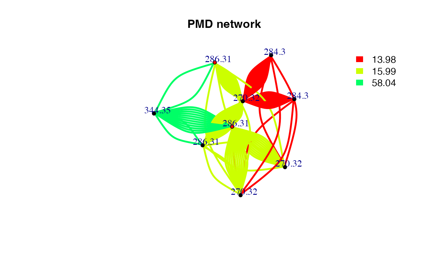
# Consider the correlation coefficient cutoff
chain <- getchain(spmeinvivo,diff = c(2.02,14.02,15.99,58.04,13.98),mass = 286.3101,digits = 2,corcutoff = 0.6)
# show as network
net <- graph_from_data_frame(chain$sdac,directed = F)
pal <- grDevices::rainbow(5)
plot(net,vertex.label=round(as.numeric(V(net)$name),2),vertex.size =5,edge.width = 3,edge.color = pal[as.numeric(as.factor(E(net)$diff2))],vertex.label.dist=1,vertex.color=ifelse(round(as.numeric(V(net)$name),4) %in% 286.3101,'red','black'), main = 'PMD network')
legend("topright",bty = "n",
       legend=unique(E(net)$diff2),
       fill=unique(pal[as.numeric(as.factor(E(net)$diff2))]), border=NA,horiz = F)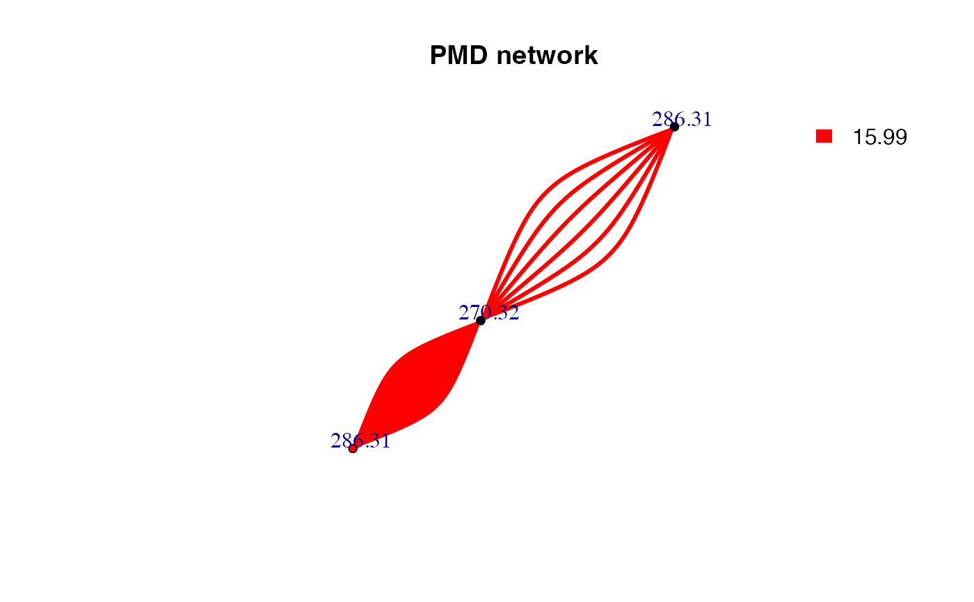
Here only three PMD relationship could be found for C18H39NO. The duplicate edges between two vertices or self-loop edges mean isomer related PMD reactions. If we consider the correlation, the network would be trimmed. Since reaction might not always involve correlation, PMD network analysis could found more potential metabolites.
If you want to see all the independent peaks’ high frequency PMDs as networks for certain sample, the following code will help. This part will use the high frequency PMDs cutoff 12 from the data to build the networks for all the independent peaks.
std <- globalstd(spmeinvivo,sda = F)
#> 75 retention time clusters found.
#> Using ng = 15
#> 5 unique PMDs retained.
#> The unique within RT clusters high frequency PMD(s) is(are)  28.03 21.98 44.03 17.03 18.01.
#> 409 isotope peaks found.
#> 109 multiple charged isotope peaks found.
#> 4 multiple charged peaks found.
#> 346 paired peaks found.
#> 8 group(s) have single peaks 14 23 32 33 54 55 56 75
#> 11 group(s) with multiple peaks while no isotope/paired relationship 4 5 7 8 11 ... 42 49 68 72 73
#> 9 group(s) with isotope without paired relationship 2 9 22 26 52 62 64 66 70
#> 4 group(s) with paired without isotope relationship 1 10 15 18
#> 43 group(s) with both paired and isotope relationship 3 6 12 13 16 ... 65 67 69 71 74
#> 291 standard masses identified.
sda <- getsda(std,freqcutoff = 12)
#> 8 groups were found as high frequency PMD group.
#> 0 was found as high frequency PMD.
#> 2.02 was found as high frequency PMD.
#> 13.98 was found as high frequency PMD.
#> 14.05 was found as high frequency PMD.
#> 15.99 was found as high frequency PMD.
#> 28.03 was found as high frequency PMD.
#> 30.05 was found as high frequency PMD.
#> 126.14 was found as high frequency PMD.
df <- sda$sda
net <- graph_from_data_frame(df,directed = F)
pal <- grDevices::rainbow(length(unique(E(net)$diff2)))
plot(net,vertex.label=NA,vertex.size = 5,edge.width = 3,edge.color = pal[as.numeric(as.factor(E(net)$diff2))],main = 'PMD network')
legend("topright",bty = "n",
       legend=unique(E(net)$diff2),
       fill=unique(pal[as.numeric(as.factor(E(net)$diff2))]), border=NA,horiz = F)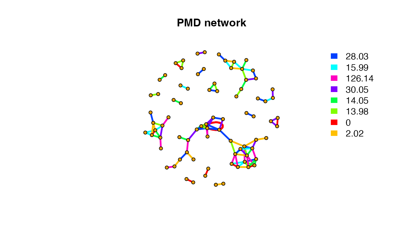
Here we could find clusters of metabolites. We could detect such network community structure.
# network community structure detection
ceb <- cluster_edge_betweenness(net,weights = abs(E(net)$cor), directed = F)
#> Warning in cluster_edge_betweenness(net, weights = abs(E(net)$cor), directed = F): Membership vector will be selected based on the highest modularity score.
#> Source: community/edge_betweenness.c:504
plot(ceb, net,vertex.label=NA,vertex.size = 5,edge.width = 3,) 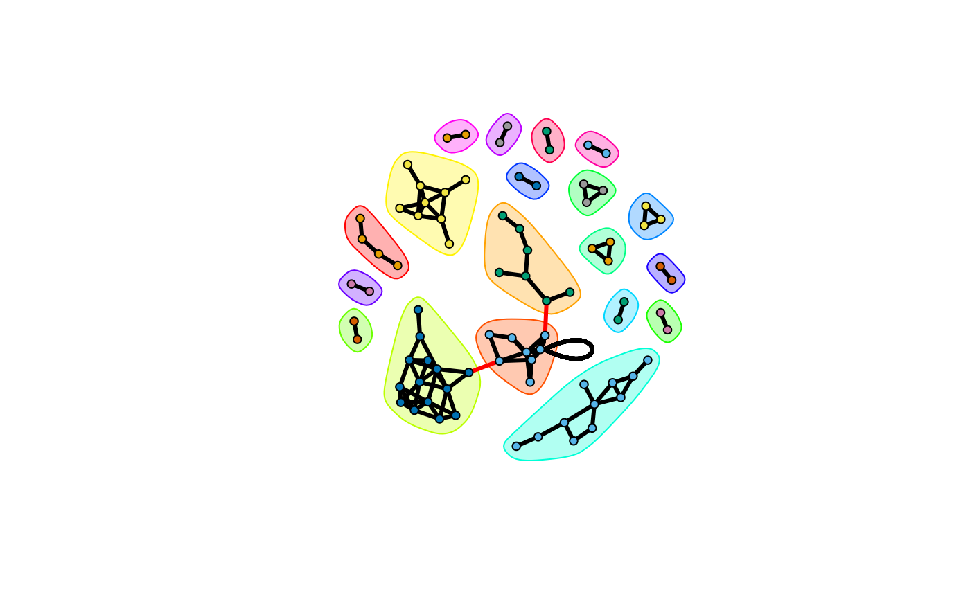
# output membership
head(cbind(ceb$membership,ceb$names))
#>      [,1] [,2]
#> [1,] "1"  "146.118268664153"
#> [2,] "1"  "162.112813715075"
#> [3,] "2"  "284.295501708984"
#> [4,] "2"  "284.295597233849"
#> [5,] "1"  "192.160430908203"
#> [6,] "3"  "326.342517752117"
Such network could also be build on correlation directed analysis which use correlation between paired peaks to build network.
cbp <- enviGCMS::getfilter(std,rowindex = std$stdmassindex)
cda <- getcda(cbp)
df <- cda$cda
# filter based on retention time differences larger than 2 mins
df <- df[df$diffrt>120,]
netc <- graph_from_data_frame(df,directed = F)
plot(netc,vertex.label=NA,vertex.size = 5,edge.width = 3,main = 'Correlation network')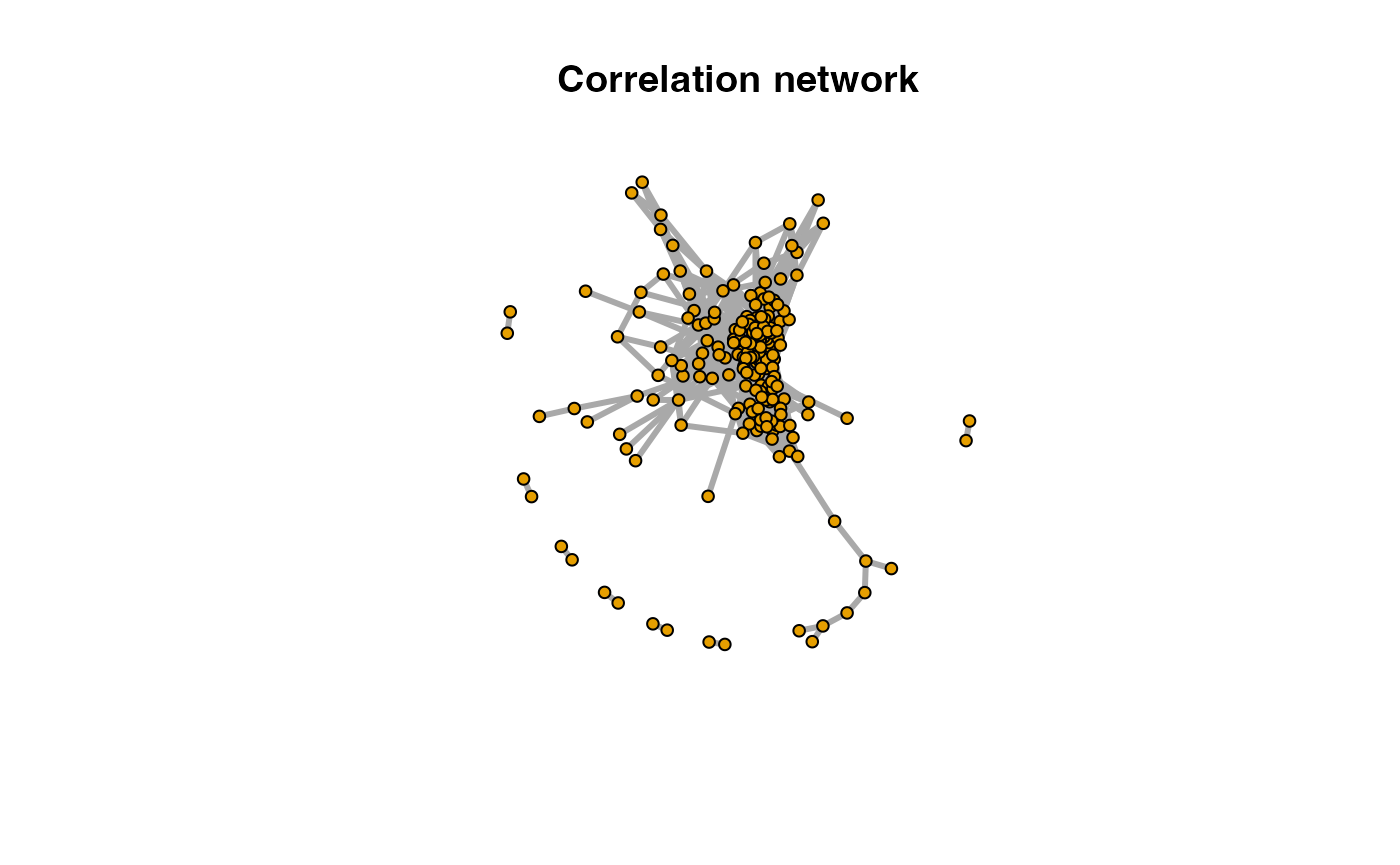
As shown above, correlation network without PMD might merge into one big network, which lose the details of chemical reactions.
Shiny application
The PMD network for certain compound could be generated by run
runPMDnet().
Tracing specific reaction paths and homologous series
For sophisticated reactomics, getchainseq allows you to
trace complex specific reaction sequences using a pattern DSL
(Domain-Specific Language), similar to regex for mass spec. The
gethomolog function provides a convenient wrapper to
extract homologous series (e.g., repeated CH2 / 14.01 units).
# Trace homologous series with 14.01 PMD (+CH2)
homo <- gethomolog(spmeinvivo, unit = 14.01)
#> Step 1 rep 1: no edges for pmd=14.01.

# Trace complex sequences e.g. oxidation (15.99) followed by multiple repeated methylation (14.01+)
sequence <- getchainseq(spmeinvivo, "15.99; 14.01+")
#> Step 2 rep 1: no edges for pmd=14.01.
Source appointment
Peaks from samples could be from endogenous compounds or exogenous compounds. However, it’s hard to tell for untargeted analysis. In terms of PMD, if one peak belongs to a high frequency PMD network, it means a relatively high activity. If such sample belongs to a biological specimen, it might be endogenous compound. If a peak show no PMD network with other peaks, the biological system might not have enzyme to make reaction happen. Exogenous compounds will show a lower degree since they are xenobiotics. Since most of the peaks will show a low degree, the median of the degree could be used as cutoff. Then we could make source appointment if the assumption is hold.
deg <- degree(net, mode = 'all')
median(deg)
#> [1] 2
endogenous <- names(deg)[deg>median(deg)]
exogenous <- names(deg)[deg<=median(deg)]
In this case, we will have 31 endogenous compounds while 51 exogenous compounds. When you find a peak show differences between groups, you could check the degree to infer its sources.
Another parameter would be the average network distances. Endogenous compounds could form a larger network with long average network distances while exogenous compounds will connected to network with small average network distances. Such parameter could be used to determine the source of unknown compound by checking the average network distances of the compounds PMD network.
Be careful, one compound could be endogenous for one sample while exogenous for another sample. In this case, PMD network would give hints on the sources based on the context of the samples.
Biomarker reaction
Biomarker always means biomarker compounds. However, if we could
quantify the reaction relationship, we could use biomarker reaction to
trace certain biological process. You could use getreact to
extract the ion pairs shared the same PMD and intensity ratio RSD% lower
than certain cutoff. Then the sum of the intensity of all PMD pairs’
ions could be used to compare the reaction level changes among
samples.
pmd <- getreact(spmeinvivo,pmd=15.99)
# show the ions with the same PMD
head(pmd$pmd)
#>         ms1      ms2     diff     rt1     rt2  diffrt rtg1 rtg2 rtgdiff
#> 5  174.1489 158.1546 15.99434 337.418 470.364 132.946   44   31      13
#> 6  175.1481 159.1575 15.99055 614.413 470.364 144.049   17   31      14
#> 12 209.1552 193.1632 15.99202 611.412 337.633 273.779   17   44      27
#> 13 211.1695 195.1745 15.99491 614.625 594.485  20.140   17   46      29
#> 16 228.1973 212.2025 15.99473 453.157 639.100 185.943   45   13      32
#> 19 244.1921 228.1973 15.99486 614.842 453.157 161.685   17   45      28
#>          cor diff2        r       rh       rl
#> 5  0.9247231 15.99 25.01946 48.53964 28.03499
#> 6  0.9164059 15.99 18.12926 35.13135 25.48822
#> 12 0.7567381 15.99 29.09434 38.95531 41.61674
#> 13 0.7378409 15.99 26.62548 33.46165 61.56227
#> 16 0.9749689 15.99  6.76019 30.01754 26.76093
#> 19 0.9670674 15.99 17.96722 42.20945 30.01754
# show the corresponding quantitative PMD data across samples, each row show the sum of intensity of paired masses qualified for stable mass pairs
head(pmd$pmddata)
#>           1405_Fish1_F1 1405_Fish1_F2 1405_Fish1_F3 1405_Fish2_F1 1405_Fish2_F2
#> 174.1/337     18327.863     11388.643     15368.711      9068.557     19759.098
#> 175.1/614      6746.288      4237.569      6581.992      3085.251      6108.837
#> 209.2/611     30644.459     19496.458     33519.253     11647.966     31169.817
#> 211.2/615      5958.334      4270.901      6285.724      2757.028      6065.346
#> 228.2/453     29245.928     21199.245     38668.407     16822.114     36020.058
#> 244.2/615     41582.379     30025.253     57302.819     20846.835     51716.437
#>           1405_Fish2_F3 1405_Fish3_F1 1405_Fish3_F2 1405_Fish3_F3
#> 174.1/337     12995.786     16878.397     18647.770     25557.292
#> 175.1/614      3420.075      6435.200      7535.579      8806.608
#> 209.2/611     14064.021     29421.515     38893.482     43313.165
#> 211.2/615      3041.366      5809.946      8795.206      8089.021
#> 228.2/453     19484.297     32281.370     36797.052     39304.713
#> 244.2/615     24315.314     45535.922     59156.064     61720.089
If your data don’t have retention time, reaction level change can also be checked.
spmeinvivo$rt <- NULL
pmd <- getreact(spmeinvivo,pmd=15.99)
# show the ions with the same PMD
head(pmd$pmd)
#>         ms1      ms2     diff       cor diff2        r       rh       rl
#> 5  174.1489 158.1546 15.99434 0.9247231 15.99 25.01946 48.53964 28.03499
#> 6  175.1481 159.1575 15.99055 0.9164059 15.99 18.12926 35.13135 25.48822
#> 12 209.1552 193.1632 15.99202 0.7567381 15.99 29.09434 38.95531 41.61674
#> 13 211.1695 195.1745 15.99491 0.7378409 15.99 26.62548 33.46165 61.56227
#> 16 228.1973 212.2025 15.99473 0.9749689 15.99  6.76019 30.01754 26.76093
#> 19 244.1921 228.1973 15.99486 0.9670674 15.99 17.96722 42.20945 30.01754
# show the corresponding quantitative PMD data across samples, each row show the sum of intensity of paired masses qualified for stable mass pairs
head(pmd$pmddata)
#>           1405_Fish1_F1 1405_Fish1_F2 1405_Fish1_F3 1405_Fish2_F1 1405_Fish2_F2
#> 174.1/337     18327.863     11388.643     15368.711      9068.557     19759.098
#> 175.1/614      6746.288      4237.569      6581.992      3085.251      6108.837
#> 209.2/611     30644.459     19496.458     33519.253     11647.966     31169.817
#> 211.2/615      5958.334      4270.901      6285.724      2757.028      6065.346
#> 228.2/453     29245.928     21199.245     38668.407     16822.114     36020.058
#> 244.2/615     41582.379     30025.253     57302.819     20846.835     51716.437
#>           1405_Fish2_F3 1405_Fish3_F1 1405_Fish3_F2 1405_Fish3_F3
#> 174.1/337     12995.786     16878.397     18647.770     25557.292
#> 175.1/614      3420.075      6435.200      7535.579      8806.608
#> 209.2/611     14064.021     29421.515     38893.482     43313.165
#> 211.2/615      3041.366      5809.946      8795.206      8089.021
#> 228.2/453     19484.297     32281.370     36797.052     39304.713
#> 244.2/615     24315.314     45535.922     59156.064     61720.089
Now we have two methods to compute the quantitative PMD responses and user should select method depending on research purposes. ‘static’ will only consider the stable mass pairs across samples and such reactions will be limited by the enzyme or other factors than substrates. ‘dynamic’ will consider the unstable paired masses by normalization the relatively unstable peak with stable peak between paired masses and such reactions will be limited by one or both peaks in the paired masses.
data("spmeinvivo")
pmd <- getreact(spmeinvivo,pmd=15.99,method = 'dynamic')
# show the ions with the same PMD
head(pmd$pmd)
#>         ms1      ms2     diff      rt1      rt2  diffrt rtg1 rtg2 rtgdiff
#> 1  147.9900 132.0050 15.98503 145.0880  49.4910 95.5970   20    4      16
#> 2  162.1128 146.1183 15.99455 256.1585 288.1300 31.9715    5   23      18
#> 3  172.1705 156.1777 15.99279 478.9360 405.3890 73.5470   43   30      13
#> 9  177.0914 161.0967 15.99477 574.3390 490.7225 83.6165   39   37       2
#> 10 183.0809 167.0901 15.99080 533.7950 511.2940 22.5010   48   12      36
#> 11 184.9858 168.9988 15.98695  85.4930 135.4660 49.9730    2   41      39
#>            cor diff2         r        rh       rl
#> 1   0.41231393 15.99  34.86972 27.176089 39.84553
#> 2   0.95185232 15.99  30.42748 89.272157 84.24422
#> 3   0.64609844 15.99  56.74081 50.385313 42.86262
#> 9  -0.07743575 15.99 100.61906  8.080905 43.90465
#> 10  0.54183684 15.99  38.29089 16.749724 42.53298
#> 11 -0.36694067 15.99  46.87352 18.159277 40.61084
# show the corresponding quantitative PMD data across samples, each row show the sum of intensity of paired masses qualified for stable mass pairs
head(pmd$pmddata)
#>   1405_Fish1_F1 1405_Fish1_F2 1405_Fish1_F3 1405_Fish2_F1 1405_Fish2_F2
#> 1    0.01999437   0.016242675    0.01880472   0.006371798   0.024304585
#> 2    1.53528194   0.962295635    1.10219074   0.982190726   1.604363528
#> 3    0.46404167   1.194387570    1.06934597   0.250054581   0.509676599
#> 4    1.20386141   1.669736528    1.32468366   1.213218611   1.083057203
#> 5    0.01461837   0.006770954    0.01055026   0.009490853   0.008958319
#> 6    9.26463385  12.763610562    3.97502609  14.657795223   4.041131973
#>   1405_Fish2_F3 1405_Fish3_F1 1405_Fish3_F2 1405_Fish3_F3
#> 1    0.01309609   0.011523649   0.011596937   0.017668097
#> 2    1.43917818   1.064822325   1.846236771   2.609787311
#> 3    1.01508469   0.406659176   0.874861257   0.621074214
#> 4    2.05169832   7.765315730   0.832736564   2.117740805
#> 5    0.01549754   0.007511291   0.005490916   0.005883117
#> 6    9.12757512   7.779539564   7.970752923   4.004298286
You can also output the quantitative results of all high frequency PMDs existing in the data.
data("spmeinvivo")
# remove redundant peaks
list <- globalstd(spmeinvivo,sda = T)
#> 75 retention time clusters found.
#> Using ng = 15
#> 5 unique PMDs retained.
#> The unique within RT clusters high frequency PMD(s) is(are)  28.03 21.98 44.03 17.03 18.01.
#> 409 isotope peaks found.
#> 109 multiple charged isotope peaks found.
#> 4 multiple charged peaks found.
#> 346 paired peaks found.
#> 8 group(s) have single peaks 14 23 32 33 54 55 56 75
#> 11 group(s) with multiple peaks while no isotope/paired relationship 4 5 7 8 11 ... 42 49 68 72 73
#> 9 group(s) with isotope without paired relationship 2 9 22 26 52 62 64 66 70
#> 4 group(s) with paired without isotope relationship 1 10 15 18
#> 43 group(s) with both paired and isotope relationship 3 6 12 13 16 ... 65 67 69 71 74
#> 291 standard masses identified.
#> PMD frequency cutoff is 6 by PMD network analysis with largest network average distance 6.67 .
#> 53 groups were found as high frequency PMD group.
#> 0 was found as high frequency PMD.
#> 1.98 was found as high frequency PMD.
#> 2.01 was found as high frequency PMD.
#> 2.02 was found as high frequency PMD.
#> 6.97 was found as high frequency PMD.
#> 11.96 was found as high frequency PMD.
#> 12 was found as high frequency PMD.
#> 13.98 was found as high frequency PMD.
#> 14.02 was found as high frequency PMD.
#> 14.05 was found as high frequency PMD.
#> 15.99 was found as high frequency PMD.
#> 16.03 was found as high frequency PMD.
#> 19.04 was found as high frequency PMD.
#> 28.03 was found as high frequency PMD.
#> 30.05 was found as high frequency PMD.
#> 31.99 was found as high frequency PMD.
#> 33.02 was found as high frequency PMD.
#> 37.02 was found as high frequency PMD.
#> 42.05 was found as high frequency PMD.
#> 48.04 was found as high frequency PMD.
#> 48.98 was found as high frequency PMD.
#> 49.02 was found as high frequency PMD.
#> 54.05 was found as high frequency PMD.
#> 56.06 was found as high frequency PMD.
#> 56.1 was found as high frequency PMD.
#> 58.04 was found as high frequency PMD.
#> 58.08 was found as high frequency PMD.
#> 58.11 was found as high frequency PMD.
#> 63.96 was found as high frequency PMD.
#> 66.05 was found as high frequency PMD.
#> 68.06 was found as high frequency PMD.
#> 70.04 was found as high frequency PMD.
#> 70.08 was found as high frequency PMD.
#> 74.02 was found as high frequency PMD.
#> 80.03 was found as high frequency PMD.
#> 82.08 was found as high frequency PMD.
#> 88.05 was found as high frequency PMD.
#> 91.1 was found as high frequency PMD.
#> 93.12 was found as high frequency PMD.
#> 94.1 was found as high frequency PMD.
#> 96.09 was found as high frequency PMD.
#> 101.05 was found as high frequency PMD.
#> 108.13 was found as high frequency PMD.
#> 110.11 was found as high frequency PMD.
#> 112.16 was found as high frequency PMD.
#> 116.08 was found as high frequency PMD.
#> 122.15 was found as high frequency PMD.
#> 124.16 was found as high frequency PMD.
#> 126.14 was found as high frequency PMD.
#> 144.18 was found as high frequency PMD.
#> 148.04 was found as high frequency PMD.
#> 150.2 was found as high frequency PMD.
#> 173.18 was found as high frequency PMD.
newlist <- enviGCMS::getfilter(list,rowindex = list$stdmassindex)
# get high frequency pmd
hfpmd <- unique(newlist$sda$diff2)
# generate quantitative results
pmd <- getreact(newlist,pmd=hfpmd)
# output the kegg pmd in the data
table(pmd$pmd$diff2)
#>
#>      0   1.98   2.01   2.02   6.97  11.96     12  13.98  14.02  14.05  15.99
#>      1      3      2      6      1      1      3      4      3      6      3
#>  16.03  19.04  28.03  30.05  31.99  33.02  42.05  48.04  48.98  49.02  54.05
#>      3      2      5      1      2      1      2      1      1      3      1
#>  56.06  58.04  58.08  63.96  66.05  68.06  70.04  70.08  74.02  80.03  82.08
#>      1      6      1      2      2      1      1      2      7      3      2
#>  88.05   91.1  93.12   94.1  96.09 101.05 108.13 110.11 112.16 116.08 122.15
#>      3      2      3      2      1      1      2      3      4      6      2
#> 124.16 126.14 148.04
#>      3      6      2
# output quantitative result for each PMD
head(pmd$pmddata)
#>           1405_Fish1_F1 1405_Fish1_F2 1405_Fish1_F3 1405_Fish2_F1 1405_Fish2_F2
#> 200.2/522      76781.54      40625.84      77922.53     28510.920      79221.24
#> 228.2/453      38231.65      26164.21      44139.68     21243.456      45048.10
#> 240.2/639      31881.67      19485.44      31170.56     13105.650      33620.20
#> 268.3/639      39620.62      22678.74      40315.71     19270.755      39626.76
#> 254.2/639      27475.32      16563.06      26416.10     12568.091      26500.43
#> 261.2/557      24604.42      14415.48      21970.93      9424.969      25368.75
#>           1405_Fish2_F3 1405_Fish3_F1 1405_Fish3_F2 1405_Fish3_F3
#> 200.2/522      40736.98      68844.35      83690.73      91978.11
#> 228.2/453      26938.08      40441.85      45445.05      52223.88
#> 240.2/639      20422.46      29060.96      32886.11      39062.02
#> 268.3/639      24927.91      36500.59      41108.70      48308.70
#> 254.2/639      15106.66      27064.28      30026.87      32384.46
#> 261.2/557      11698.38      21809.08      37162.69      37774.73
# output quantitative result for unique PMD
upmd <- aggregate(pmd$pmddata, by=list(pmd$pmd$diff2),sum)
# column for samples and row for unique PMD
head(upmd)
#>   Group.1 1405_Fish1_F1 1405_Fish1_F2 1405_Fish1_F3 1405_Fish2_F1 1405_Fish2_F2
#> 1    0.00      72539.75      46921.79      83489.08      28793.02      80299.40
#> 2    1.98     112810.76      66245.18     146623.69      47083.72     139250.82
#> 3    2.01     221243.45      93950.41     271935.00      52129.93     225979.34
#> 4    2.02    8315494.48    6518031.80    8671833.02    5135730.18    8679495.21
#> 5    6.97      26432.13      20929.65      35015.28      16707.43      33324.33
#> 6   11.96     214066.24     112212.13     270152.44      79751.55     240539.00
#>   1405_Fish2_F3 1405_Fish3_F1 1405_Fish3_F2 1405_Fish3_F3
#> 1      35190.01      73796.58     101046.21     105464.49
#> 2      63606.69     127173.02     148943.11     149585.77
#> 3      89406.65     141388.51     155992.98     166769.47
#> 4    6196265.89    8057717.46    8798917.44    9524655.11
#> 5      19249.17      30033.02      33716.19      34905.22
#> 6     104862.63     211044.91     265591.16     314792.74
You can also output the quantitative results of all PMDs existing in current KEGG database.
# output all existing PMD in KEGG
keggpmd <- unique(round(keggrall$pmd,2))
data("spmeinvivo")
# remove redundant peaks
list <- globalstd(spmeinvivo)
#> 75 retention time clusters found.
#> Using ng = 15
#> 5 unique PMDs retained.
#> The unique within RT clusters high frequency PMD(s) is(are)  28.03 21.98 44.03 17.03 18.01.
#> 409 isotope peaks found.
#> 109 multiple charged isotope peaks found.
#> 4 multiple charged peaks found.
#> 346 paired peaks found.
#> 8 group(s) have single peaks 14 23 32 33 54 55 56 75
#> 11 group(s) with multiple peaks while no isotope/paired relationship 4 5 7 8 11 ... 42 49 68 72 73
#> 9 group(s) with isotope without paired relationship 2 9 22 26 52 62 64 66 70
#> 4 group(s) with paired without isotope relationship 1 10 15 18
#> 43 group(s) with both paired and isotope relationship 3 6 12 13 16 ... 65 67 69 71 74
#> 291 standard masses identified.
newlist <- enviGCMS::getfilter(list,rowindex = list$stdmassindex)
# generate quantitative results
pmd <- getreact(newlist,pmd=keggpmd)
# output the kegg pmd in the data
table(pmd$pmd$diff2)
#>
#>      0   0.04   1.98   2.02   2.04   2.98   3.05   3.98   4.03      6   6.05
#>      1      3      3      6      1      1      2      1      1      1      2
#>   7.03   7.06    7.2   9.95   9.98  10.02  11.96     12  12.04  12.07  12.95
#>      1      1      1      1      2      1      1      3      2      1      1
#>  12.99  13.03  13.98  14.02  14.05     15  15.01  15.02  15.05  15.79  15.94
#>      2      1      4      3      6      1      1      1      1      1      1
#>  15.99     16  16.01  16.03  16.09  16.93     17  17.03  17.99  18.01  18.06
#>      3      2      1      3      1      1      3      1      2      1      1
#>     19  19.04  19.87  20.06     21  21.98  22.05  22.76   22.8     24  25.02
#>      1      2      1      1      1      1      1      1      2      3      1
#>  25.98  26.02  26.06     28  28.03  28.07   28.1  28.99  29.03  29.96     31
#>      3      5      1      2      5      2      1      1      1      1      3
#>  31.01  31.04  31.95  31.99  33.93  34.01  34.02  34.31  35.02  35.03  38.06
#>      1      2      1      2      1      2      2      1      1      1      1
#>  39.99  40.03  40.07  40.96  42.01  42.05  42.08  43.01  43.17  45.03  45.06
#>      1      3      1      1      1      2      2      1      1      1      2
#>  45.96  46.04  47.94     48  50.02  51.05  52.01  52.07  53.05  55.06  56.03
#>      1      1      2      2      1      1      1      2      3      1      1
#>  56.04  56.06  56.27  56.94  57.02  57.06  57.97  58.04  58.08  58.75  59.04
#>      1      1      1      1      1      2      1      6      1      1      2
#>  60.08  61.02  61.22  63.03  63.96  64.02  64.03  66.05  67.03  67.07  68.03
#>      1      3      1      1      2      1      1      2      4      1      2
#>  68.06  70.01  70.04  71.04  71.98     74  75.03  75.05  75.34  77.03  77.05
#>      1      1      1      1      1      2      1      1      2      1      1
#>  78.09  78.96  79.04  80.03  80.06  80.83  81.95  81.97  82.04  82.09  83.07
#>      2      2      1      3      1      1      1      1      1      1      1
#>  84.02  84.06  86.11  88.02  88.05  90.05  90.14  90.55  93.02  93.04  94.02
#>      1      1      2      1      3      3      1      1      1      1      2
#>  94.12  94.31  95.04  95.97     98  98.07  98.08  98.14 100.08 100.95 101.05
#>      1      2      1      1      2      2      1      2      1      1      1
#> 101.96 102.01 102.14 102.25 102.97 103.03 103.27 103.83 103.91 103.99 104.06
#>      1      1      1      1      1      1      1      1      1      1      2
#> 106.03 108.02 108.06 108.09 108.13 109.03 109.05 110.04 110.83 112.12 113.07
#>      1      1      1      1      2      1      1      1      1      1      1
#> 115.83 116.95 117.06 118.03 119.04 119.06 120.06 121.87 122.01 122.02 123.01
#>      1      1      3      1      1      1      2      1      1      1      1
#> 123.99 125.02 125.88 126.03  126.1 126.18 126.96 127.12 128.01 128.12 129.08
#>      1      1      2      1      2      2      1      3      1      1      1
#> 130.85 131.09 131.86 132.94    135 135.96 137.06 139.96 142.04 142.75 142.97
#>      1      1      1      1      1      2      1      1      1      1      1
#>  143.1 143.94 144.04 144.06 145.04 146.06    147 149.94 150.07 152.12    154
#>      2      1      1      1      1      1      1      1      1      1      1
#> 157.01 157.05 157.11 158.02 158.13 158.17 158.95 159.09 159.14 160.16 161.15
#>      1      1      1      1      1      1      2      1      1      1      1
#> 161.95 162.03 162.05 163.09 165.06 168.02 168.07    170 172.05 177.06 178.18
#>      1      1      1      1      2      1      1      1      1      1      1
#> 182.17 183.13 186.03 191.99 193.01 194.04 194.24 195.02 195.03 197.05 198.01
#>      1      2      1      1      1      1      1      1      1      1      1
#> 199.96 200.18 201.04 204.19 206.06 206.08 207.02  210.2 215.05 215.97 217.07
#>      1      1      1      2      1      1      2      3      1      1      1
#> 218.17  222.2 229.04 230.09 236.93 241.05 243.02 249.09 250.09 252.22 252.92
#>      1      1      1      1      1      1      1      1      1      1      1
#> 265.03 268.22  269.1 275.12 278.02 278.16 289.17  291.1    297 300.08  300.9
#>      1      1      1      1      2      1      1      1      1      1      1
#> 301.91 302.95 304.08 306.17 311.87 315.18  316.9  339.1 343.71 344.95 345.86
#>      1      1      1      1      1      2      1      1      1      1      1
#> 346.74 348.01 349.89  369.8 375.91 381.02 390.28 405.02 409.03 409.42 409.98
#>      1      1      1      1      1      1      1      1      1      1      1
#> 431.06 437.11 439.02 440.89 447.07 454.17  454.3 455.05 456.23 463.06  466.1
#>      1      1      1      1      1      1      1      1      1      1      1
#> 472.97 473.05 475.05 476.07 478.04 488.07 501.07 501.08 505.13 516.12 517.06
#>      1      1      1      1      1      1      1      1      1      1      1
#> 518.06 526.05 537.08 546.13 546.98 552.06 554.09 586.06 599.18 612.56
#>      1      1      1      1      1      1      1      1      1      1
# output quantitative result for each PMD
head(pmd$pmddata)
#>           1405_Fish1_F1 1405_Fish1_F2 1405_Fish1_F3 1405_Fish2_F1 1405_Fish2_F2
#> 159/155       35181.202     38958.595     32009.376     51346.078     28559.260
#> 636.2/819     45321.672     33160.944     70592.139     26804.485     70922.188
#> 173.1/611     21060.045     12412.283     21212.641      8046.332     19278.585
#> 577.1/820      2860.706      1645.137      3285.761      1937.062      3347.514
#> 593.2/819      6353.084      4155.004      8805.660      3774.374      8029.871
#> 159/155       25512.422     38824.191     33660.574     48794.630     20651.311
#>           1405_Fish2_F3 1405_Fish3_F1 1405_Fish3_F2 1405_Fish3_F3
#> 159/155       41888.784     29068.087     25006.374     33043.005
#> 636.2/819     33615.276     29465.045     65983.634     82993.419
#> 173.1/611      8715.165     19432.080     24901.629     26559.379
#> 577.1/820      2016.036      2521.557      3219.349      4223.686
#> 593.2/819      4331.519      5995.990      7702.984     11416.088
#> 159/155       40127.066     35015.350     29515.079     30543.740
# output quantitative result for unique PMD
upmd <- aggregate(pmd$pmddata, by=list(pmd$pmd$diff2),sum)
# column for samples and row for unique PMD
head(upmd)
#>   Group.1 1405_Fish1_F1 1405_Fish1_F2 1405_Fish1_F3 1405_Fish2_F1 1405_Fish2_F2
#> 1    0.00     72539.754     46921.790     83489.076     28793.020     80299.395
#> 2    0.04    172890.767    102824.406    209381.165     67517.693    200256.694
#> 3    1.98    112810.762     66245.180    146623.690     47083.719    139250.821
#> 4    2.02   8315494.479   6518031.801   8671833.018   5135730.184   8679495.213
#> 5    2.04      5588.112      2835.595      6882.802      1988.072      4584.455
#> 6    2.98     70741.800     36761.679     71959.565     29974.327     78883.528
#>   1405_Fish2_F3 1405_Fish3_F1 1405_Fish3_F2 1405_Fish3_F3
#> 1     35190.011     73796.583    101046.212    105464.491
#> 2     87815.305    184631.030    232005.956    239070.075
#> 3     63606.694    127173.025    148943.105    149585.769
#> 4   6196265.889   8057717.463   8798917.442   9524655.115
#> 5      2931.107      4411.049      5688.054      5438.388
#> 6     40546.116     62671.685     79751.686     82474.088
Reactomics analysis for MS only data
When retention time is not provided, m/z vector can still be used to
check reaction level changes. You might use getrda to find
the high frequency PMDs.
data(spmeinvivo)
# get the m/z
mz <- spmeinvivo$mz
# get the m/z intensity for all m/z, the row order is the same with mz
insms <- spmeinvivo$data
# check high frequency pmd
sda <- getrda(mz)
#> 164462 pmd found.
#> 20 pmd used.
colnames(sda)
#>  [1] "0"       "1.001"   "1.002"   "1.003"   "1.004"   "2.015"   "2.016"
#>  [8] "14.015"  "17.026"  "18.011"  "21.982"  "28.031"  "28.032"  "44.026"
#> [15] "67.987"  "67.988"  "88.052"  "116.192" "135.974" "135.975"
# save them as numeric vector
hfpmd <- as.numeric(colnames(sda))
Then getpmddf function can be used to extract all the
paired ions for certain PMD.
# get details for certain pmd
pmddf <- getpmddf(mz,pmd=18.011,digits = 3)
# add intensity for all the paired ions
mz1ins <- insms[match(pmddf$ms1,mz),]
mz2ins <- insms[match(pmddf$ms2,mz),]
# get the pmd pair intensity
pmdins <- mz1ins+mz2ins
# get the pmd total intensity across samples
pmdinsall <- apply(pmdins,2,sum)
# show the PMD intensity
pmdinsall
#> 1405_Fish1_F1 1405_Fish1_F2 1405_Fish1_F3 1405_Fish2_F1 1405_Fish2_F2
#>       9898514       7801273      10363201       5847334      10479551
#> 1405_Fish2_F3 1405_Fish3_F1 1405_Fish3_F2 1405_Fish3_F3
#>       7021375      10584976      12989961      12559649
You can also calculate the static or dynamic PMD intensity for m/z only data.
# get the ratio of larger m/z over smaller m/z
ratio <- mz2ins/mz1ins
# filter PMD based on RSD% across samples
# cutoff 30%
cutoff <- 0.3
# get index for static PMD
rsdidx <- apply(ratio,1,function(x) sd(x)/mean(x)<cutoff)
# get static PMD
pmddfstatic <- pmddf[rsdidx,]
# get static intensity
pmdinsstatic <- pmdins[rsdidx,]
# normalize the ions pair intensity to avoid influences from large response factors
pmdinsstaticscale <- t(scale(t(pmdinsstatic)))
# get the pmd static intensity across samples
pmdinsstaticall <- apply(pmdinsstaticscale,2,sum)
# show the PMD static intensity for each sample
pmdinsstaticall
#> 1405_Fish1_F1 1405_Fish1_F2 1405_Fish1_F3 1405_Fish2_F1 1405_Fish2_F2
#>      1.027100    -16.703628      2.373645    -27.241358     12.433566
#> 1405_Fish2_F3 1405_Fish3_F1 1405_Fish3_F2 1405_Fish3_F3
#>    -17.757951      7.924290     19.802820     18.141514

# get index for dynamic PMD
rsdidx <- apply(ratio,1,function(x) sd(x)/mean(x)>=cutoff)
# get dynamic PMD
pmddfdynamic <- pmddf[rsdidx,]
# get dynamic intensity for ms1 and ms2
pmdinsdynamicms1 <- apply(mz1ins[rsdidx,],1,function(x) sd(x)/mean(x))
pmdinsdynamicms2 <- apply(mz2ins[rsdidx,],1,function(x) sd(x)/mean(x))
# find the stable ms and use ratio as intensity
idx <- pmdinsdynamicms1>pmdinsdynamicms2
pmdinsdynamic <- ratio[rsdidx,]
pmdinsdynamic[idx,] <- 1/ratio[rsdidx,][idx,]
# get the pmd dynamic intensity across samples
pmdinsdynamicall <- apply(pmdinsdynamic,2,sum)
# show the PMD dynamic intensity for each sample
pmdinsdynamicall
#> 1405_Fish1_F1 1405_Fish1_F2 1405_Fish1_F3 1405_Fish2_F1 1405_Fish2_F2
#>      374.1957      315.6090      388.0063      207.8236      233.4380
#> 1405_Fish2_F3 1405_Fish3_F1 1405_Fish3_F2 1405_Fish3_F3
#>      199.9064      283.4682      327.9651      256.2044
You can also use getpmddf function extract all the
paired ions for multiple PMDs. Then you could generate the network based
on the output.
# get details for certain pmd
pmddf <- getpmddf(mz,pmd=hfpmd,digits = 3)
# viz by igraph package
library(igraph)
net <- graph_from_data_frame(pmddf,directed = F)
pal <- grDevices::rainbow(length(unique(E(net)$diff2)))
plot(net,vertex.label=NA,vertex.size = 5,edge.width = 3,edge.color = pal[as.numeric(as.factor(E(net)$diff2))],main = 'PMD network')
legend("topright",bty = "n",
       legend=unique(E(net)$diff2),
       fill=unique(pal[as.numeric(as.factor(E(net)$diff2))]), border=NA,horiz = F)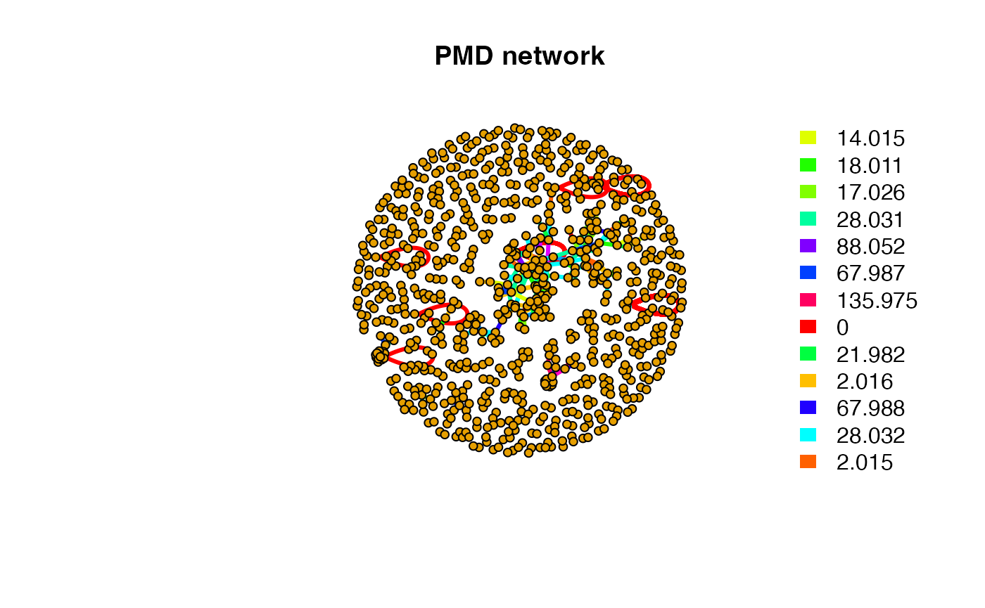
If you prefer to get a pmd network for a specific mass. You can still
use getchain function.
data(spmeinvivo)
spmeinvivo$rt <- NULL
chain <- getchain(spmeinvivo,diff = c(2.02,14.02,15.99,58.04,13.98),mass = 286.3101,digits = 2,corcutoff = 0)
# show as network
net <- graph_from_data_frame(chain$sdac,directed = F)
pal <- grDevices::rainbow(5)
plot(net,vertex.label=round(as.numeric(V(net)$name),2),vertex.size =5,edge.width = 3,edge.color = pal[as.numeric(as.factor(E(net)$diff2))],vertex.label.dist=1,vertex.color=ifelse(round(as.numeric(V(net)$name),4) %in% 286.3101,'red','black'), main = 'PMD network')
legend("topright",bty = "n",
       legend=unique(E(net)$diff2),
       fill=unique(pal[as.numeric(as.factor(E(net)$diff2))]), border=NA,horiz = F)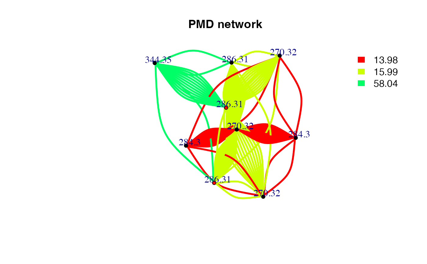
PMD Reaction Database
To check the pmd reaction database:
# all reaction
data("omics")
head(omics)
#>   X   KEGG RHEA_ID DIRECTION MASTER_ID   ec ecocyc macie
#> 1 1 R00001   22455        BI     22452 <NA>   <NA>  <NA>
#> 2 2 R00004   24579        BI     24576 <NA>   <NA>  <NA>
#> 3 3 R00005   19032        BI     19029 <NA>   <NA>  <NA>
#> 4 4 R00008   22751        BI     22748 <NA>   <NA>  <NA>
#> 5 5 R00009   20312        BI     20309 <NA>   <NA>  <NA>
#> 6 6 R00010   20871        BI     20868 <NA>   <NA>  <NA>
#>                   metacyc reactome
#> 1 ENDOPOLYPHOSPHATASE-RXN     <NA>
#> 2   INORGPYROPHOSPHAT-RXN     <NA>
#> 3                    <NA>     <NA>
#> 4                    <NA>     <NA>
#> 5                    <NA>     <NA>
#> 6                    <NA>     <NA>
#>                                                compounds     pmd
#> 1  [phosphate](n+1) + n H2O <=> n H(+) + (n+1) phosphate      NA
#> 2               diphosphate + H2O <=> H(+) + 2 phosphate      NA
#> 3 3 H(+) + H2O + urea-1-carboxylate <=> 2 CO2 + 2 NH4(+)      NA
#> 4       4-hydroxy-4-methyl-2-oxoglutarate <=> 2 pyruvate      NA
#> 5                                  2 H2O2 <=> 2 H2O + O2      NA
#> 6            alpha,alpha-trehalose + H2O <=> 2 D-glucose 162.053
# kegg reaction
data("keggrall")
head(keggrall)
#>      rid              rc                      ez      ms1      formula1
#> 1 R00002         RC00002                1.18.6.1 506.9957 C10H16N5O13P3
#> 2 R00010         RC00049                3.2.1.28 342.1162     C12H22O11
#> 3 R00012         RC00002                2.7.7.45 522.9907 C10H16N5O14P3
#> 4 R00014 RC00027;RC02744 1.2.4.1;2.2.1.6;4.1.1.1 425.0450 C12H19N4O7P2S
#> 5 R00015 RC00077;RC00247                2.4.1.99 342.1162     C12H22O11
#> 6 R00015 RC00077;RC00247                2.4.1.99 342.1162     C12H22O11
#>        ms2       formula2     pmd  C  H O N P S
#> 1 427.0294  C10H15N5O10P2  79.966  0  1 3 0 1 0
#> 2 180.0634        C6H12O6 162.053  6 10 5 0 0 0
#> 3 868.0381 C20H28N10O21P4 345.047 10 12 7 5 1 0
#> 4 469.0712  C14H23N4O8P2S  44.026  2  4 1 0 0 0
#> 5 180.0634        C6H12O6 162.053  6 10 5 0 0 0
#> 6 504.1690      C18H32O16 162.053  6 10 5 0 0 0
# literature reaction for mass spectrometry
data("sda")
head(sda)
#>         PMD                                                          origin
#> 1  0.984016                    OH ↔ NH2, e.g. de-amidiation, CHNO compounds
#> 2  1.995663 F ↔ OH, halogen exchange with hydroxy group (typically -F + OH)
#> 3  2.015650                         ± 2H, opening or forming of double bond
#> 4  7.004671                       F ↔ CN, halogen exchange with cyano group
#> 5  8.965779                      Cl ↔ CN, halogen exchange with cyano group
#> 6 13.979265               O ↔ 2H, e.g. Oxidation follwed by H2O elimination
#>                                            Ref. mode
#> 1 https://doi.org/10.1016/S1044-0305(99)00090-2    b
#> 2 https://doi.org/10.1016/S1044-0305(99)00090-2    e
#> 3 https://doi.org/10.1016/S1044-0305(99)00090-2    b
#> 4 https://doi.org/10.1016/S1044-0305(99)00090-2    e
#> 5 https://doi.org/10.1016/S1044-0305(99)00090-2    e
#> 6 https://doi.org/10.1016/S1044-0305(99)00090-2    b
To check the HMDB pmd database:
data("hmdb")
head(hmdb)
#> C H O N P S pmd pmd2 percentage
#> 1 -3 4 2 0 0 0 0.021 0.02 0.9623060
#> 2 1 4 -1 0 0 0 0.036 0.04 0.9503645
#> 3 5 4 -4 0 0 0 0.052 0.05 0.9412861
#> 4 2 8 -2 0 0 0 0.073 0.07 0.9617834
#> 5 6 8 -5 0 0 0 0.088 0.09 0.9247730
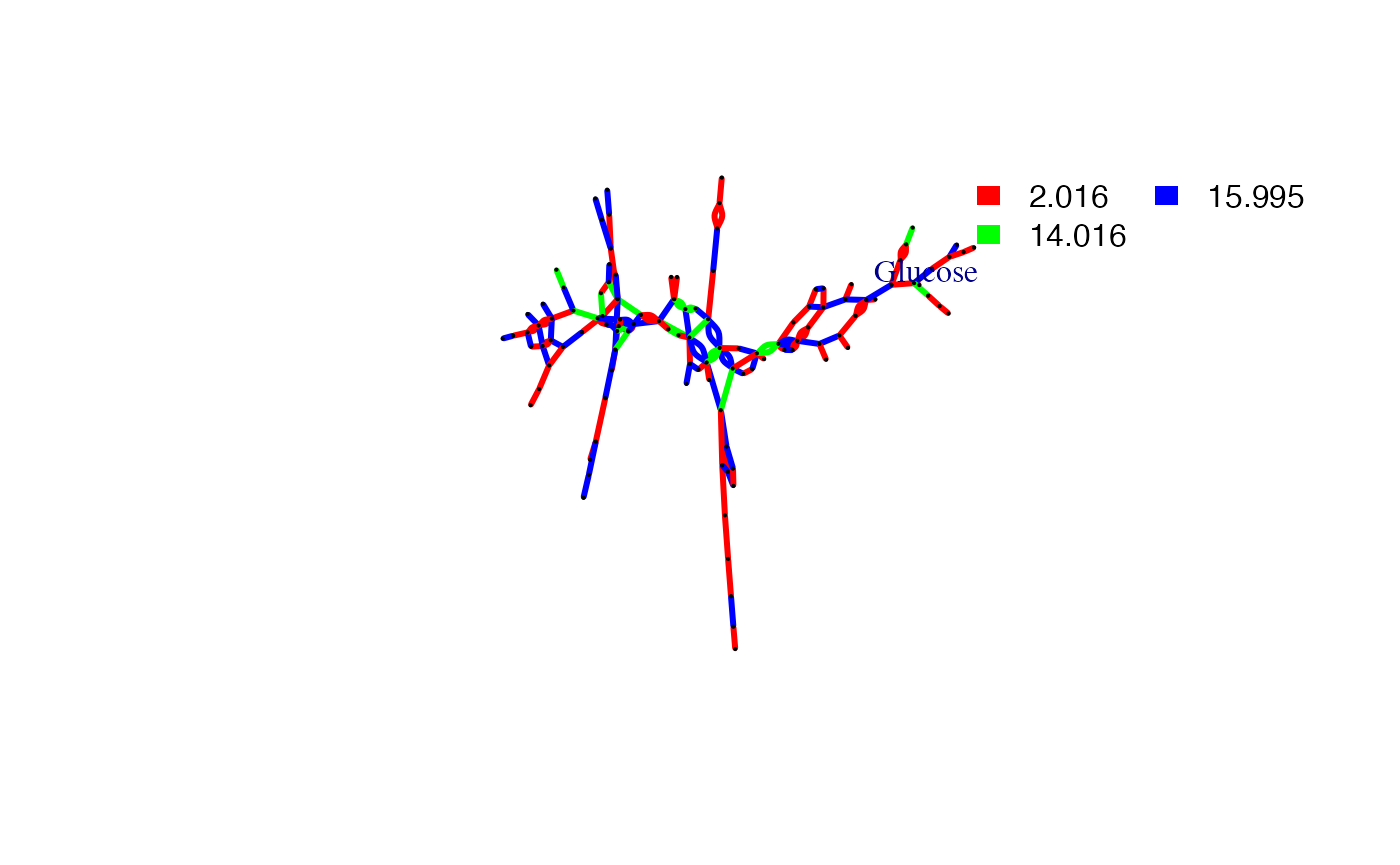
#> 6 -1 12 0 0 0 0 0.094 0.09 0.9648936To extract any compound KEGG compound’s pmd network with known PMD:
plotcn('C6H12O6','Glucose',c(2.016,14.016,15.995))
#> Average distance of PMD network is 9.42710759198882
#> Average degree 2.8421052631579