Paired Mass Distance(PMD) analysis for GC/LC-MS based non-targeted analysis

Introduction of Paired Mass Distance analysis

pmd package use Paired Mass Distance (PMD) relationship to analysis the GC/LC-MS based non-targeted data. PMD means the distance between two masses or mass to charge ratios. In mass spectrometry, PMD would keep the same value between two masses and two mass to charge ratios(m/z). There are two kinds of PMD involved in this package: PMD from the same compound and PMD from different compounds. In GC/LC-MS or XCMS based non-targeted data analysis, peaks could be separated by chronograph and same compound means ions from similar retention times or ions co-eluted by certain column.

PMD from the same compound

For MS1 full scan data, we could build retention time(RT) bins to assign peaks into different RT groups by retention time hierarchical clustering analysis. For each RT group, the peaks should come from same compounds or co-elutes. If certain PMD appeared in multiple RT groups, it would be related to the relationship about adducts, neutral loss, isotopologues or common fragments ions.

PMD from different compounds

The peaks from different retention time groups would like to be different compounds separated by chronograph. The PMD would reflect the relationship about homologous series or chemical reactions.

GlobalStd algorithm use the PMD within same RT group to find independent peaks among certain data set. Then, structure/reaction directed analysis use PMD from different RT groups to screen important compounds or reactions.

Data format

The input data should be a list object with at least two elements from a peaks list:

mass to charge ratio with name of mz, high resolution mass spectrometry is required
retention time with name of rt

However, I suggested to add intensity and group information to the list for validation of PMD analysis.

In this package, a data set from in vivo solid phase micro-extraction(SPME) was attached. This data set contain 9 samples from 3 fish with triplicates samples for each fish. Here is the data structure:

library(pmd)
data("spmeinvivo")
str(spmeinvivo)
#> List of 4
#>  $ data : num [1:1459, 1:9] 1095 10439 10154 2797 90211 ...
#>   ..- attr(*, "dimnames")=List of 2
#>   .. ..$ : chr [1:1459] "100.1/170" "100.5/86" "101/85" "103.1/348" ...
#>   .. ..$ : chr [1:9] "1405_Fish1_F1" "1405_Fish1_F2" "1405_Fish1_F3" "1405_Fish2_F1" ...
#>  $ group:'data.frame':   9 obs. of  2 variables:
#>   ..$ sample_name : chr [1:9] "1405_Fish1_F1" "1405_Fish1_F2" "1405_Fish1_F3" "1405_Fish2_F1" ...
#>   ..$ sample_group: chr [1:9] "fish1" "fish1" "fish1" "fish2" ...
#>  $ mz   : num [1:1459] 100 101 101 103 104 ...
#>  $ rt   : num [1:1459] 170.2 86.3 84.9 348.1 48.8 ...

You could build this list or mzrt object from the xcms objects via enviGCMS package. When you have a xcmsSet object or XCMSnExp object named xset, you could use enviGCMS::getmzrt(xset) to get such list. Of course you could build such list by yourself.

GlobalStd algorithm

GlobalStd algorithm try to find independent peaks among certain peaks list. The first step is retention time hierarchical clustering analysis. The second step is to find the relationship among adducts, neutral loss, isotopologues and common fragments ions. The third step is to screen the independent peaks.

Here is a workflow for this algorithm:

knitr::include_graphics('https://yufree.github.io/presentation/figure/GlobalStd.png')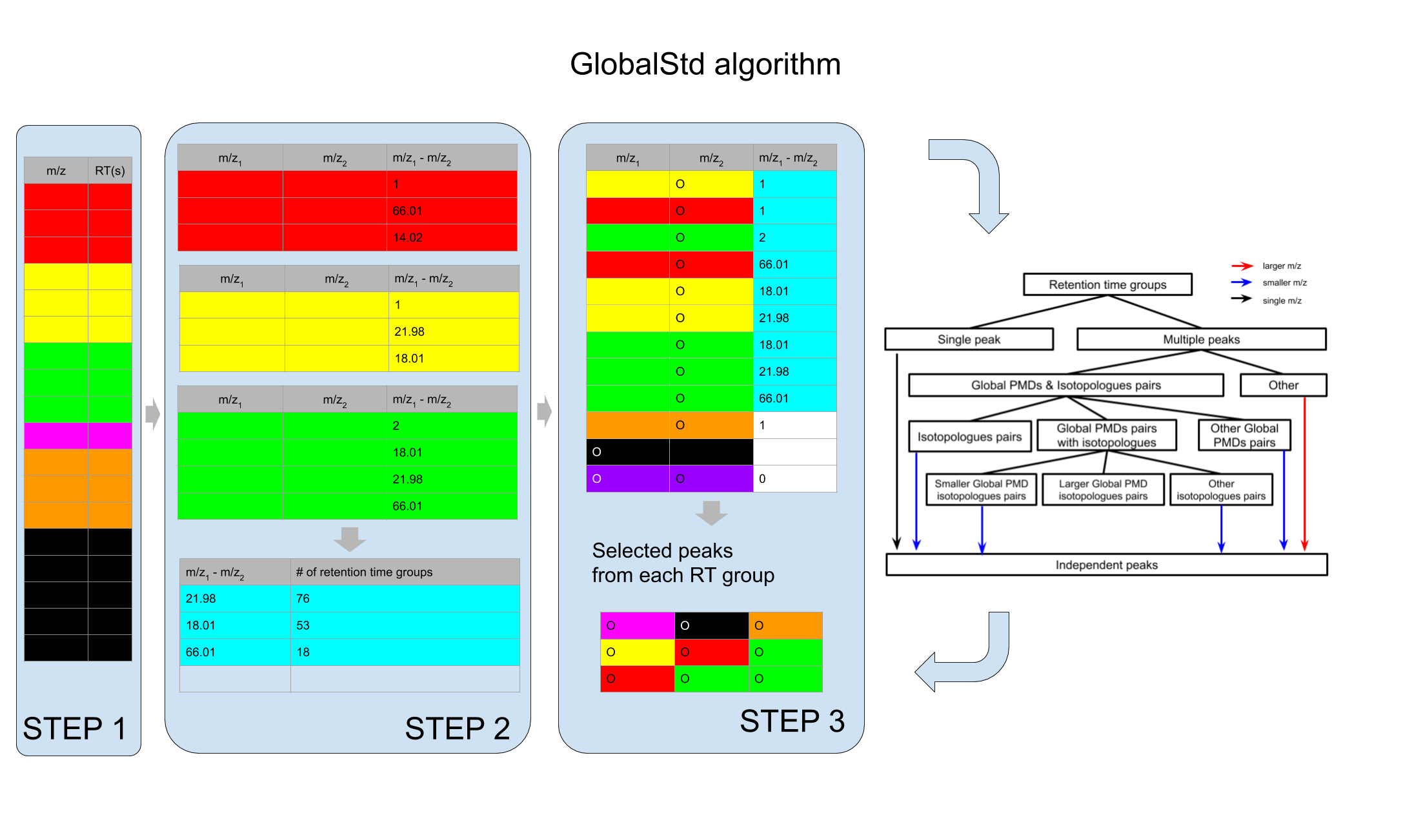

STEP1: Retention time hierarchical clustering

pmd <- getpaired(spmeinvivo)
#> 75 retention time cluster found.
#> 369 paired masses found
#> 5 unique within RT clusters high frequency PMD(s) used for further investigation.
#> The unique within RT clusters high frequency PMD(s) is(are)  28.03 21.98 44.03 17.03 18.01.
#> 719 isotopologue(s) related paired mass found.
#> 492 multi-charger(s) related paired mass found.

plotrtg(pmd)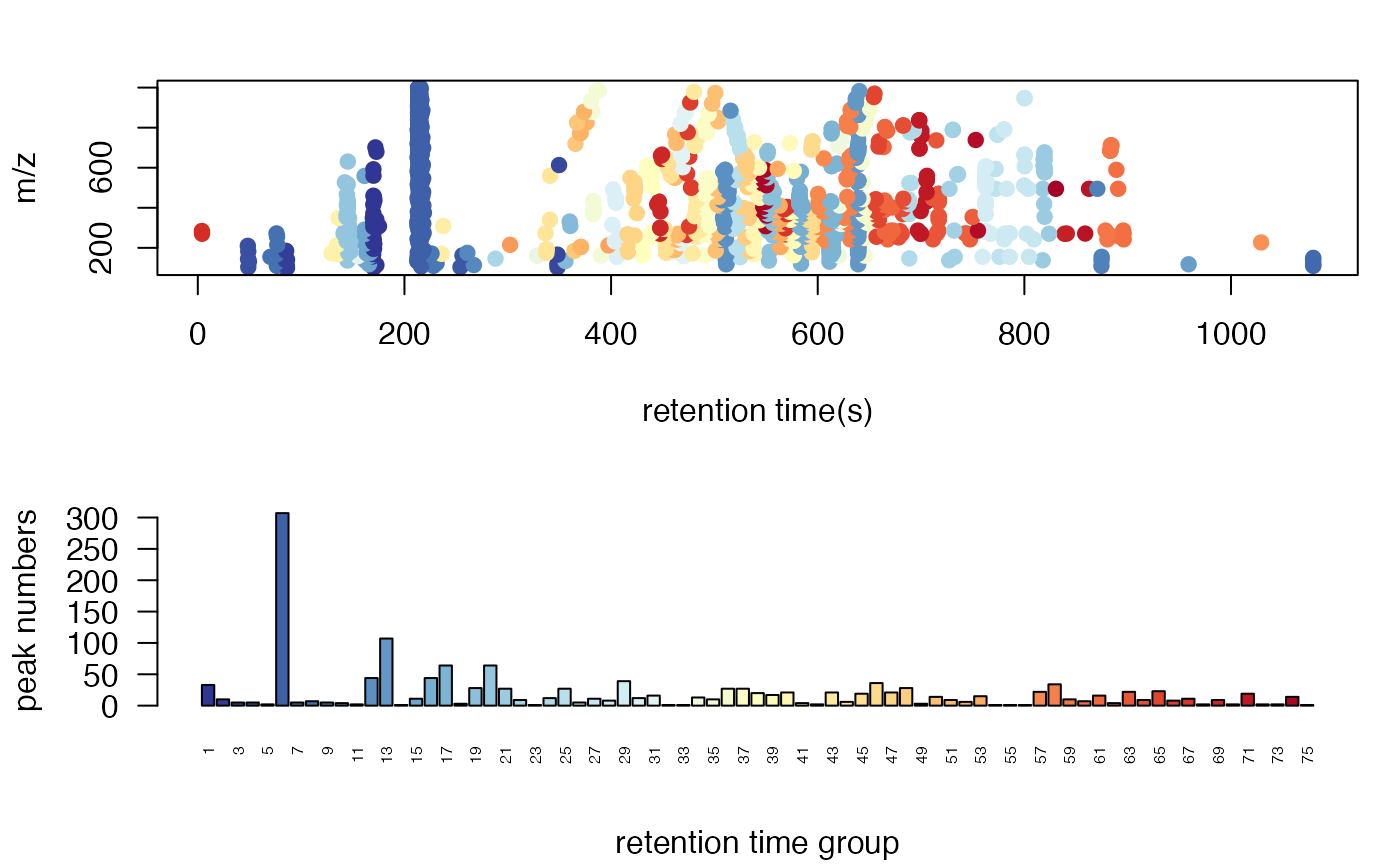

This plot would show the distribution of RT groups. The rtcutoff in function getpaired could be used to set the cutoff of the distances in retention time hierarchical clustering analysis. Retention time cluster cutoff should fit the peak picking algorithm. For HPLC, 10 is suggested and 5 could be used for UPLC.

Global PMD’s retention time group numbers should be around 20 percent of the retention time cluster numbers. For example, if you find 100 retention time clusters, I suggested you use 20 as the cutoff of empirical global PMD’s retention time group numbers. If you don’t specifically assign a value to ng, the algorithm will select such recommendation by default setting.

Take care of the retention time cluster with lots of peaks. In this case, such cluster could be co-eluted compounds on certain column. It would be wise to trim the retention time window for high quality peaks. Another important hint is that pre-filter your peak list by black samples or other quality control samples. Otherwise the running time would be long and lots of pmd relationship would be just from noise.

STEP2: Relationship among adducts, neutral loss, isotopologues and common fragments ions

The ng in function getpaired could be used to set cutoff of global PMD’s retention time group numbers. If ng is 10, at least 10 of the retention time groups should contain the shown PMD relationship. You could use plotpaired to show the distribution.

plotpaired(pmd)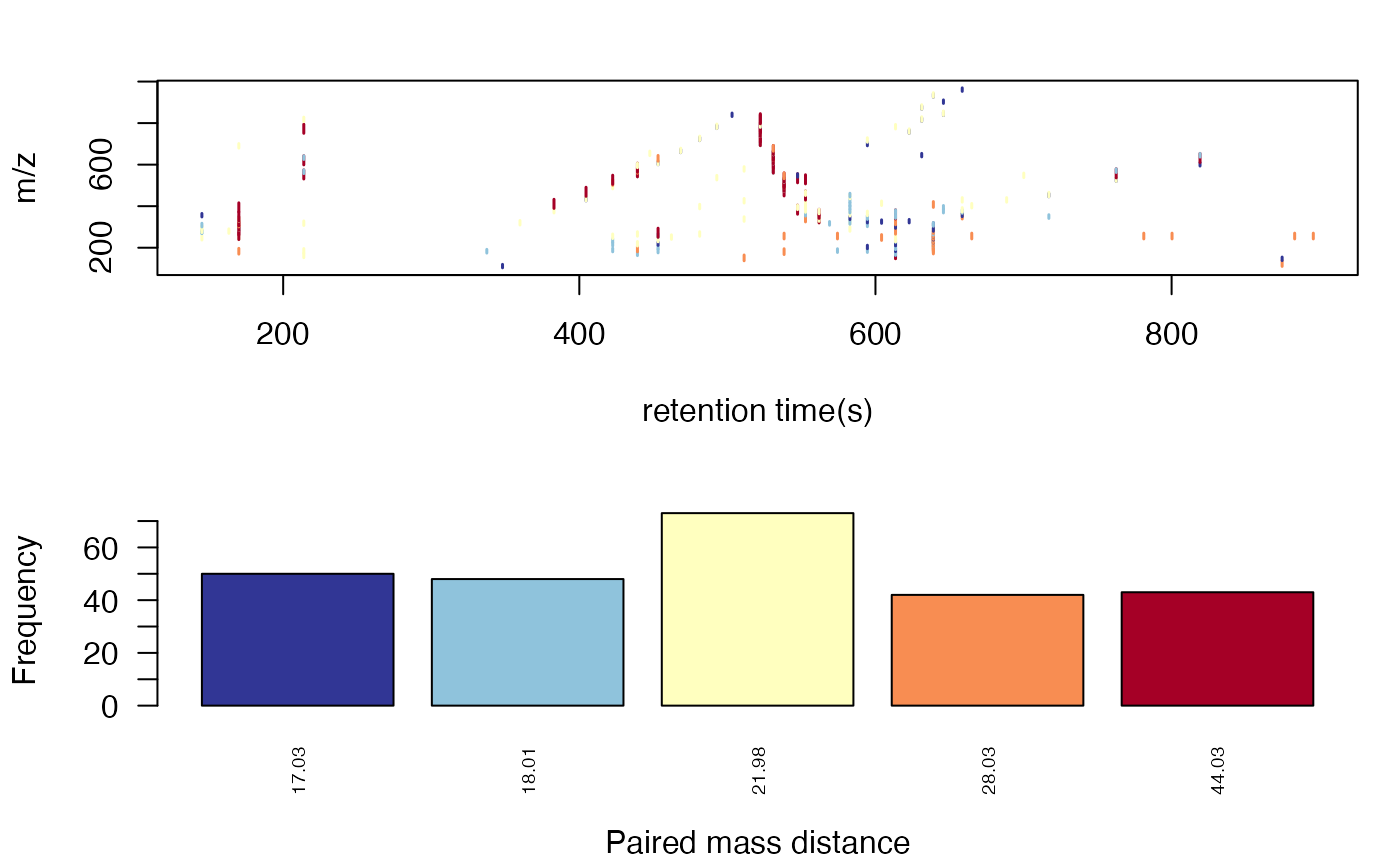

You could also show the distribution of PMD relationship by index:

# show the unique PMD found by getpaired function
for(i in 1:length(unique(pmd$paired$diff2))){
        diff <- unique(pmd$paired$diff2)[i]
        index <- pmd$paired$diff2 == diff
        plotpaired(pmd,index)
}

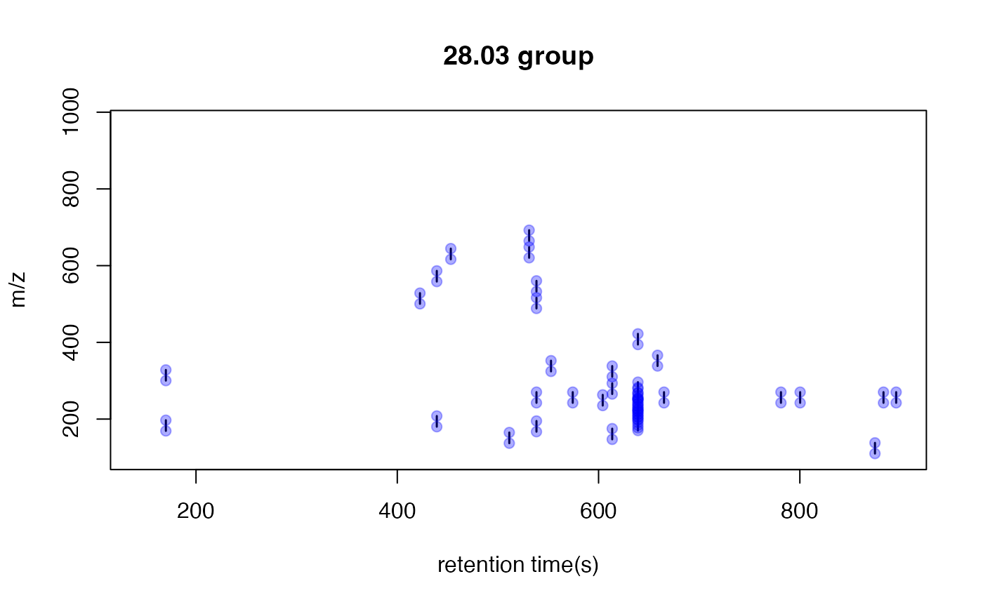
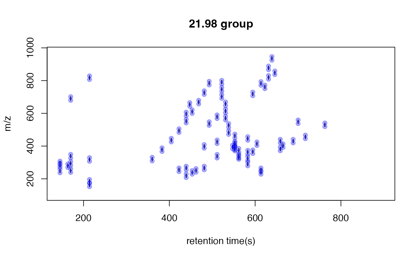
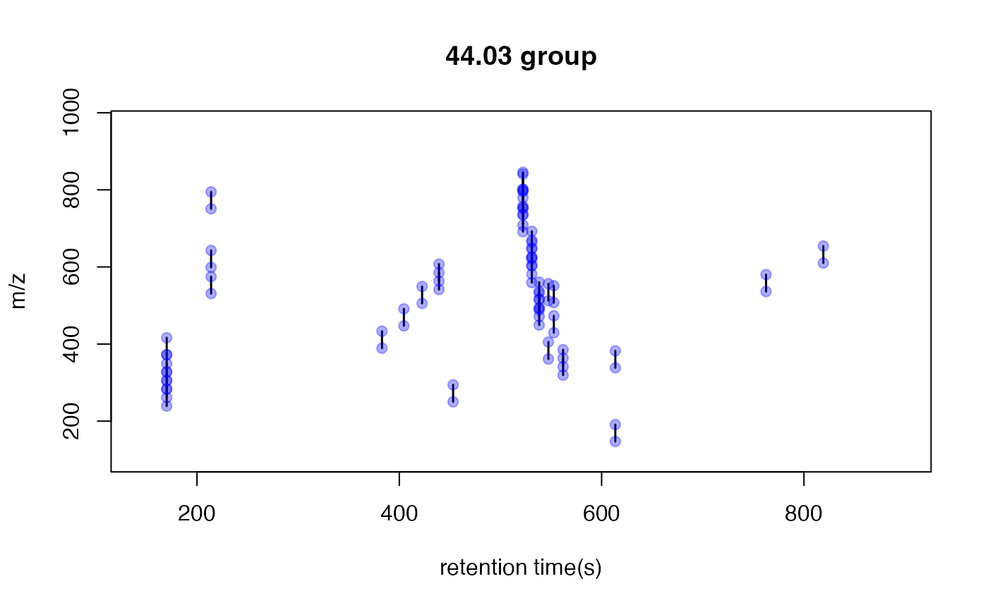
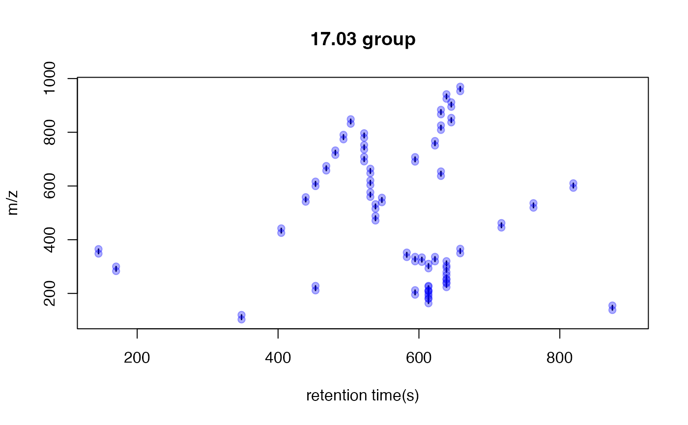
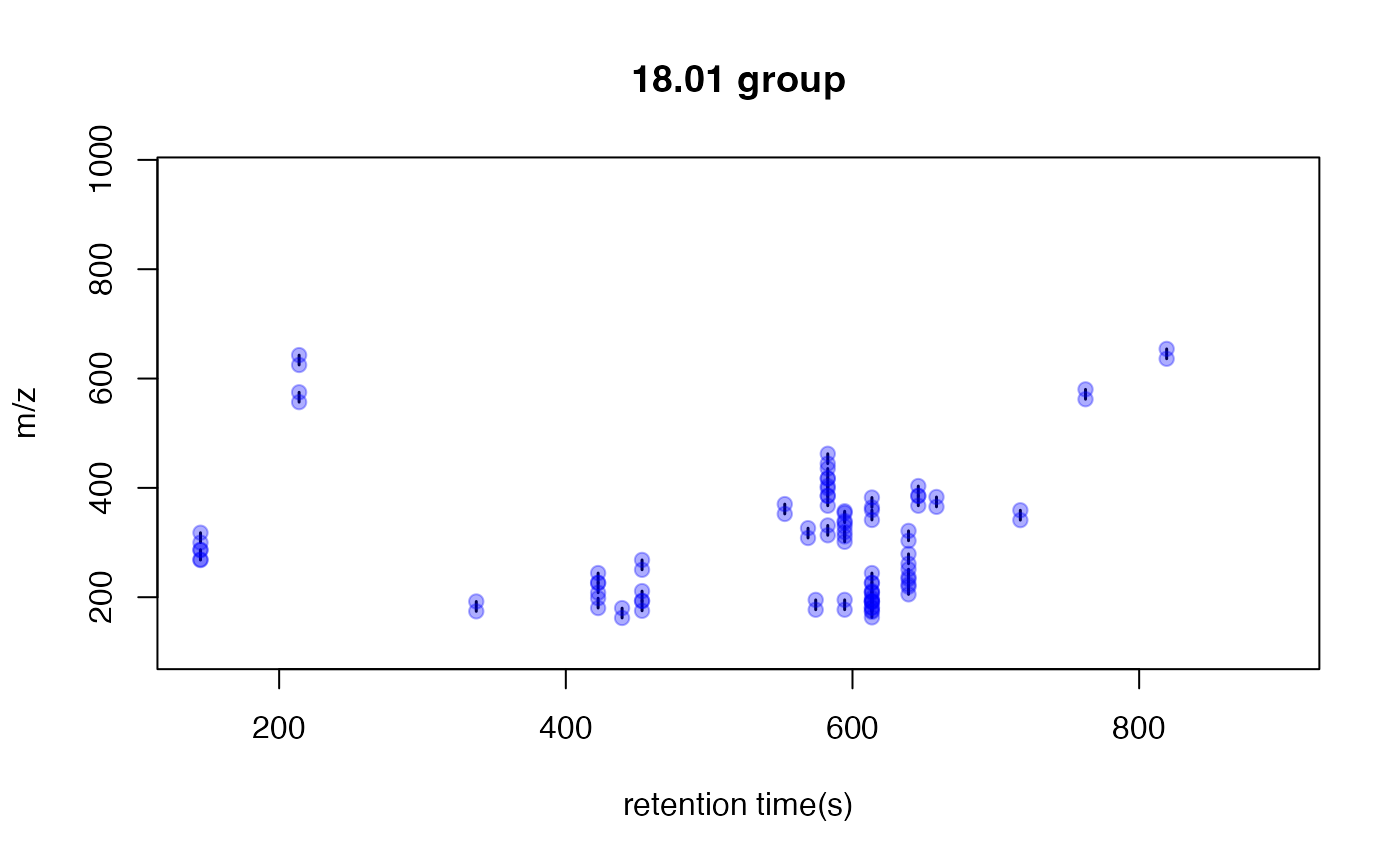
This is an easy way to find potential adducts of the data by high frequency PMD from the same compound. For example, 21.98 Da could be the mass distances between \([M+H]^+\) and \([M+Na]^+\). In this case, user could find the potential adducts or neutral loss even when they have no preferred adducts list. If one adduct exist in certain analytical system, the high frequency PMD will reveal such relationship. The high frequency PMD list could also be used to check the fragmental pattern of in-source reactions as long as such patterns are popular among all collected ions.

STEP3: Screen the independent peaks

You could use getstd function to get the independent peaks. Independent peaks mean the peaks list removing the redundant peaks such as adducts, neutral loss, isotopologues and comment fragments ions found by PMD analysis in STEP2. Ideally, those peaks could be molecular ions while they might still contain redundant peaks.

std <- getstd(pmd)
#> 8 retention group(s) have single peaks. 14 23 32 33 54 55 56 75
#> 11 group(s) with multiple peaks while no isotope/paired relationship 4 5 7 8 11 41 42 49 68 72 73
#> 9 group(s) with multiple peaks with isotope without paired relationship 2 9 22 26 52 62 64 66 70
#> 4 group(s) with paired relationship without isotope 1 10 15 18
#> 43 group(s) with paired relationship and isotope 3 6 12 13 16 17 19 20 21 24 25 27 28 29 30 31 34 35 36 37 38 39 40 43 44 45 46 47 48 50 51 53 57 58 59 60 61 63 65 67 69 71 74
#> 291 std mass found.

Here you could plot the peaks by plotstd function to show the distribution of independent peaks:

plotstd(std)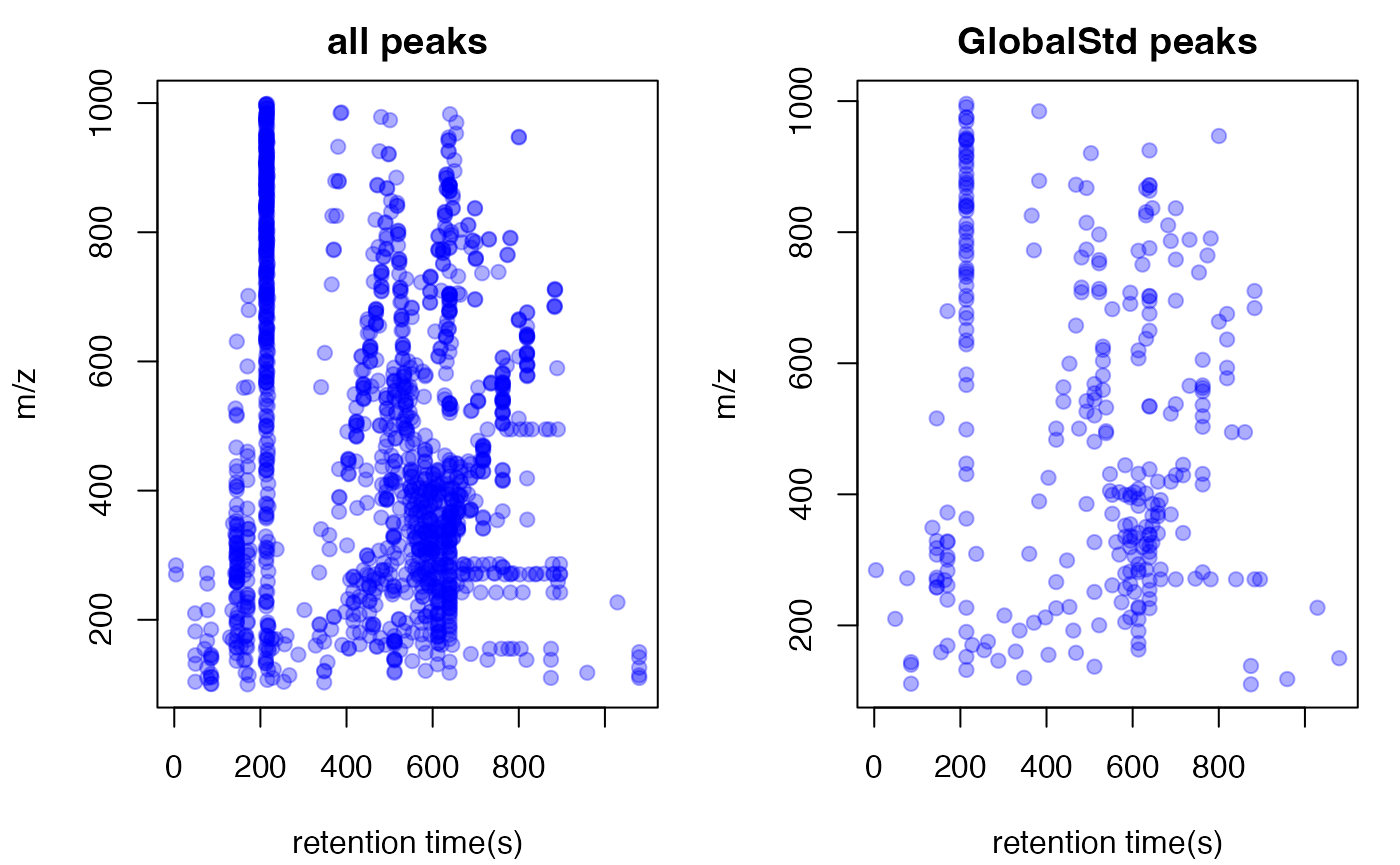

You could also plot the peaks distribution by assign a retention time group via plotstdrt:

par(mfrow = c(2,3))
plotstdrt(std,rtcluster = 23,main = 'Retention time group 23')
plotstdrt(std,rtcluster = 9,main = 'Retention time group 9')
plotstdrt(std,rtcluster = 18,main = 'Retention time group 18')
plotstdrt(std,rtcluster = 67,main = 'Retention time group 67')
plotstdrt(std,rtcluster = 49,main = 'Retention time group 49')
plotstdrt(std,rtcluster = 6,main = 'Retention time group 6')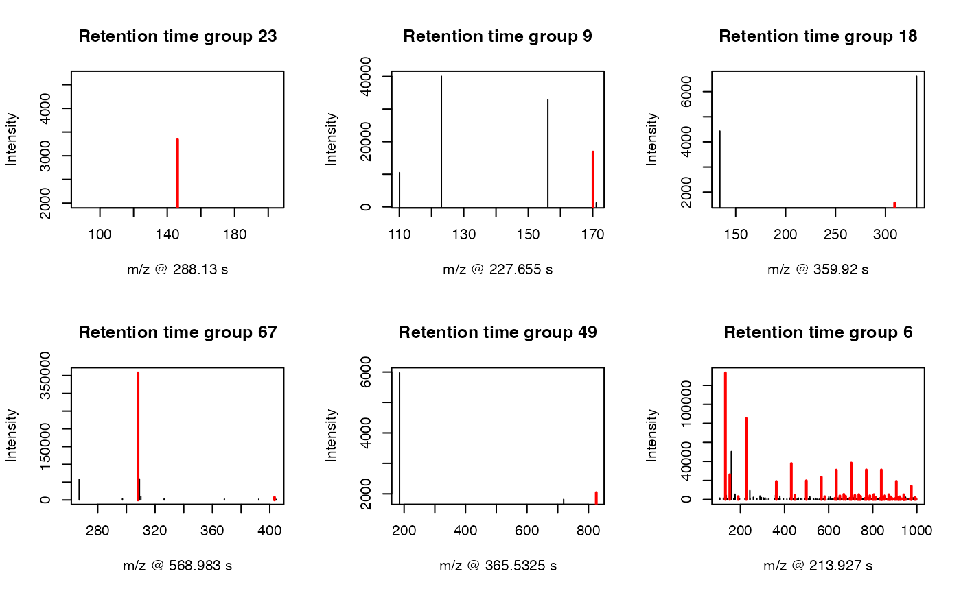

Extra filter with correlation coefficient cutoff

Original GlobalStd algorithm only use mass to charge ratio and retention time of peaks to select independent peaks. However, if intensity data across samples are available, correlation coefficient of paired ions could be used to further filter the random noise in high frequency PMDs. You could set up cutoff of Pearson Correlation Coefficient between peaks to refine the peaks selected by GlobalStd within same retention time groups. In this case, the numbers of selected independent peaks will be further reduced. When you use this parameter, make sure the intensity data are from real samples instead of blank samples, which will affect the calculation of correlation coefficient.

std2 <- getstd(pmd,corcutoff = 0.9)
#> 8 retention group(s) have single peaks. 14 23 32 33 54 55 56 75
#> 23 group(s) with multiple peaks while no isotope/paired relationship 2 4 5 7 8 10 11 15 18 26 35 39 41 42 49 50 59 62 68 69 70 72 73
#> 14 group(s) with multiple peaks with isotope without paired relationship 9 12 22 24 27 28 34 51 52 57 60 64 66 71
#> 3 group(s) with paired relationship without isotope 1 53 74
#> 27 group(s) with paired relationship and isotope 3 6 13 16 17 19 20 21 25 29 30 31 36 37 38 40 43 44 45 46 47 48 58 61 63 65 67
#> 120 std mass found.

Validation by principal components analysis(PCA)

You need to check the GlobalStd algorithm’s results by principal components analysis(PCA). If we removed too much peaks containing information, the score plot of reduced data set would show great changes.

library(enviGCMS)
par(mfrow = c(2,2),mar = c(4,4,2,1)+0.1)
plotpca(std$data,lv = as.numeric(as.factor(std$group$sample_group)),main = "all peaks")
plotpca(std$data[std$stdmassindex,],lv = as.numeric(as.factor(std$group$sample_group)),main = paste(sum(std$stdmassindex),"independent peaks"))
plotpca(std2$data[std2$stdmassindex,],lv = as.numeric(as.factor(std$group$sample_group)),main = paste(sum(std2$stdmassindex),"reduced independent peaks"))

You might find original GlobalStd algorithm show a similar PCA score plot with original data while GlobalStd algorithm considering intensity data seems change the profile. The major reason is that correlation coefficient option in the algorithm will remove the paired ions without strong correlation. It will be aggressive to remove low intensity peaks, which are vulnerable by baseline noise. However, such options would be helpful if you only concern high quality peaks for following analysis. Otherwise, original GlobalStd will keep the most information for explorer purpose.

Comparison with other pseudo spectra extraction method

GlobalStd algorithm in pmd package could be treated as a method to extract pseudo spectra. You could use getcluster to get peaks groups information for all GlobalStd peaks. This function would consider the merge of GlobalStd peaks when certain peak is involved in multiple clusters. Then you could choose export peaks with the highest intensities or base peaks in each GlobalStd merged peaks groups. Meanwhile, you could also include the correlation coefficient cutoff to further improve the data quality.

stdcluster <- getcluster(std)
# extract pseudospectra for std peak 71
idx <- unique(stdcluster$cluster$largei[stdcluster$cluster$i==71])
plot(stdcluster$cluster$mz[stdcluster$cluster$largei==idx],stdcluster$cluster$ins[stdcluster$cluster$largei==idx],type = 'h',xlab = 'm/z',ylab = 'intensity',main = 'pseudo spectra for GlobalStd peak 71')

# export peaks with the highest intensities in each GlobalStd peaks groups.
data <- stdcluster$data[stdcluster$stdmassindex2,]
# considering the correlation coefficient cutoff
stdcluster2 <- getcluster(std, corcutoff = 0.9)
# considering the correlation coefficient cutoff for both psedospectra extraction and GlobalStd algorithm
stdcluster3 <- getcluster(std2, corcutoff = 0.9)

We supplied getcorcluster to find peaks groups by correlation analysis only. The base peaks of correlation cluster were selected to stand for the compounds.

corcluster <- getcorcluster(spmeinvivo)
#> 75 retention time cluster found.

# extract pseudospectra 1@46
peak <- corcluster$cluster[corcluster$cluster$largei == '1@46',]
plot(peak$ins~peak$mz,type = 'h',xlab = 'm/z',ylab = 'intensity',main = 'pseudo spectra for correlation cluster')

Then we could compare the compare reduced result using PCA similarity factor. A good peak selection algorithm could show a high PCA similarity factor compared with original data set while retain the minimized number of peaks.

par(mfrow = c(3,3),mar = c(4,4,2,1)+0.1)
plotpca(std$data[std$stdmassindex,],lv = as.numeric(as.factor(std$group$sample_group)),main = paste(sum(std$stdmassindex),"independent peaks"))
plotpca(std$data[stdcluster$stdmassindex2,],lv = as.numeric(as.factor(std$group$sample_group)),main = paste(sum(stdcluster$stdmassindex2),"independent base peaks"))
plotpca(std$data[stdcluster2$stdmassindex2,],lv = as.numeric(as.factor(std$group$sample_group)),main = paste(sum(stdcluster2$stdmassindex2),"independent reduced base peaks"))
plotpca(std$data[corcluster$stdmassindex,],lv = as.numeric(as.factor(std$group$sample_group)),main = paste(sum(corcluster$stdmassindex),"peaks without correlationship"))
plotpca(std$data[corcluster$stdmassindex2,],lv = as.numeric(as.factor(std$group$sample_group)),main = paste(sum(corcluster$stdmassindex2),"base peaks without correlationship"))
plotpca(std$data,lv = as.numeric(as.factor(std$group$sample_group)),main = paste(nrow(std$data),"all peaks"))
plotpca(std$data[stdcluster3$stdmassindex2,],lv = as.numeric(as.factor(std$group$sample_group)),main = paste(sum(stdcluster3$stdmassindex2),"reduced independent base peaks"))
pcasf(std$data, std$data[std$stdmassindex,])
#>     pcasf 
#> 0.9993497

pcasf(std$data, std$data[stdcluster$stdmassindex2,])
#>     pcasf 
#> 0.9993578

pcasf(std$data, std$data[stdcluster2$stdmassindex2,])
#>    pcasf 
#> 0.999346

pcasf(std$data, std$data[corcluster$stdmassindex,])
#>     pcasf 
#> 0.9471586

pcasf(std$data, std$data[corcluster$stdmassindex2,])
#>     pcasf 
#> 0.9497193

pcasf(std$data, std$data[stdcluster3$stdmassindex2,])
#>    pcasf 
#> 0.713527

In this case, five peaks selection algorithms are fine to stand for the original peaks with PCA similarity score larger than 0.9. However, the independent base peaks retain the most information with relative low numbers of peaks.

Structure/Reaction directed analysis

getsda function could be used to perform Structure/reaction directed analysis. The cutoff of frequency is automate found by PMD network analysis with the largest mean distance of all nodes.

sda <- getsda(std)
#> PMD frequency cutoff is 6 by PMD network analysis with largest network average distance 6.67 .
#> 53 groups were found as high frequency PMD group.
#> 0 was found as high frequency PMD. 
#> 1.98 was found as high frequency PMD. 
#> 2.01 was found as high frequency PMD. 
#> 2.02 was found as high frequency PMD. 
#> 6.97 was found as high frequency PMD. 
#> 11.96 was found as high frequency PMD. 
#> 12 was found as high frequency PMD. 
#> 13.98 was found as high frequency PMD. 
#> 14.02 was found as high frequency PMD. 
#> 14.05 was found as high frequency PMD. 
#> 15.99 was found as high frequency PMD. 
#> 16.03 was found as high frequency PMD. 
#> 19.04 was found as high frequency PMD. 
#> 28.03 was found as high frequency PMD. 
#> 30.05 was found as high frequency PMD. 
#> 31.99 was found as high frequency PMD. 
#> 33.02 was found as high frequency PMD. 
#> 37.02 was found as high frequency PMD. 
#> 42.05 was found as high frequency PMD. 
#> 48.04 was found as high frequency PMD. 
#> 48.98 was found as high frequency PMD. 
#> 49.02 was found as high frequency PMD. 
#> 54.05 was found as high frequency PMD. 
#> 56.06 was found as high frequency PMD. 
#> 56.1 was found as high frequency PMD. 
#> 58.04 was found as high frequency PMD. 
#> 58.08 was found as high frequency PMD. 
#> 58.11 was found as high frequency PMD. 
#> 63.96 was found as high frequency PMD. 
#> 66.05 was found as high frequency PMD. 
#> 68.06 was found as high frequency PMD. 
#> 70.04 was found as high frequency PMD. 
#> 70.08 was found as high frequency PMD. 
#> 74.02 was found as high frequency PMD. 
#> 80.03 was found as high frequency PMD. 
#> 82.08 was found as high frequency PMD. 
#> 88.05 was found as high frequency PMD. 
#> 91.1 was found as high frequency PMD. 
#> 93.12 was found as high frequency PMD. 
#> 94.1 was found as high frequency PMD. 
#> 96.09 was found as high frequency PMD. 
#> 101.05 was found as high frequency PMD. 
#> 108.13 was found as high frequency PMD. 
#> 110.11 was found as high frequency PMD. 
#> 112.16 was found as high frequency PMD. 
#> 116.08 was found as high frequency PMD. 
#> 122.15 was found as high frequency PMD. 
#> 124.16 was found as high frequency PMD. 
#> 126.14 was found as high frequency PMD. 
#> 144.18 was found as high frequency PMD. 
#> 148.04 was found as high frequency PMD. 
#> 150.2 was found as high frequency PMD. 
#> 173.18 was found as high frequency PMD.

Such largest mean distance of all nodes is calculated for top 1 to 100 (if possible) high frequency PMDs. Here is a demo for the network generation process.

library(igraph)
#> 
#> Attaching package: 'igraph'
#> The following objects are masked from 'package:stats':
#> 
#>     decompose, spectrum
#> The following object is masked from 'package:base':
#> 
#>     union

cdf <- sda$sda
# get the PMDs and frequency
pmds <- as.numeric(names(sort(table(cdf$diff2),decreasing = T)))
freq <- sort(table(cdf$diff2),decreasing = T)
# filter the frequency larger than 10 for demo
pmds <- pmds[freq>10]
cdf <- sda$sda[sda$sda$diff2 %in% pmds,]
g <- igraph::graph_from_data_frame(cdf,directed = F)
l <- igraph::layout_with_fr(g)
for(i in 1:length(pmds)){
  g2 <- igraph::delete_edges(g,which(E(g)$diff2%in%pmds[1:i]))
  plot(g2,edge.width=1,vertex.label="",vertex.size=1,layout=l,main=paste('Top',length(pmds)-i,'high frequency PMDs'))
}

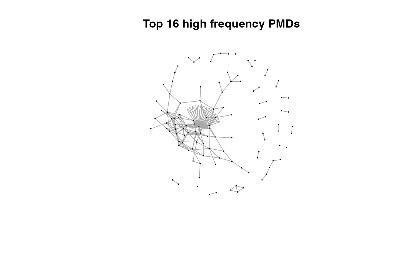
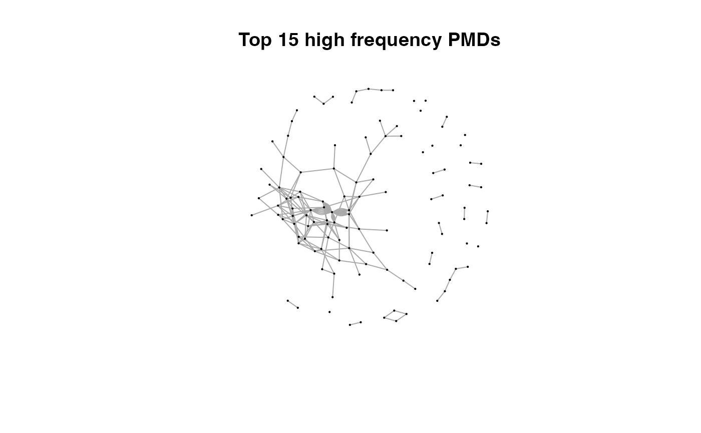
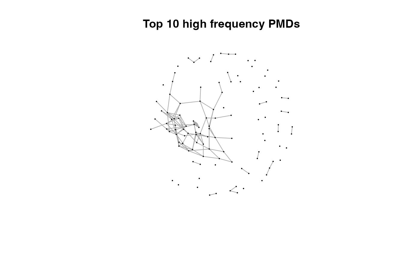
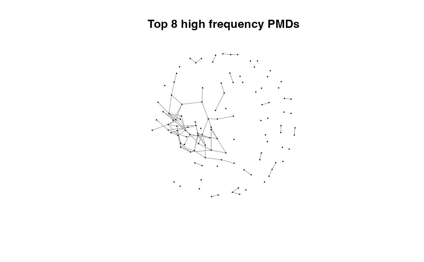
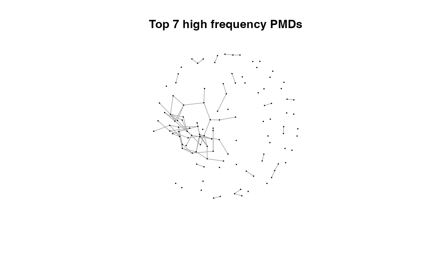
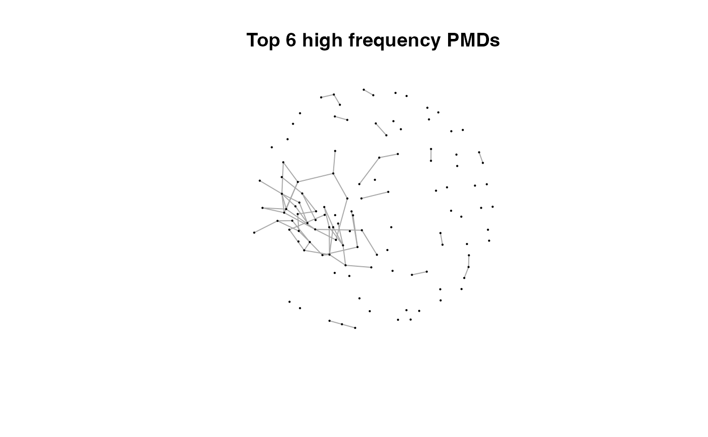
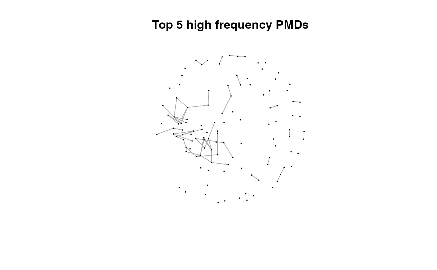
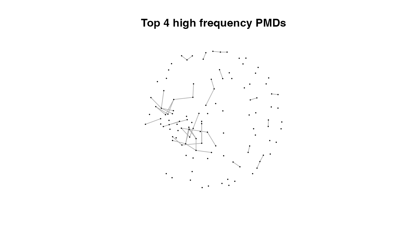
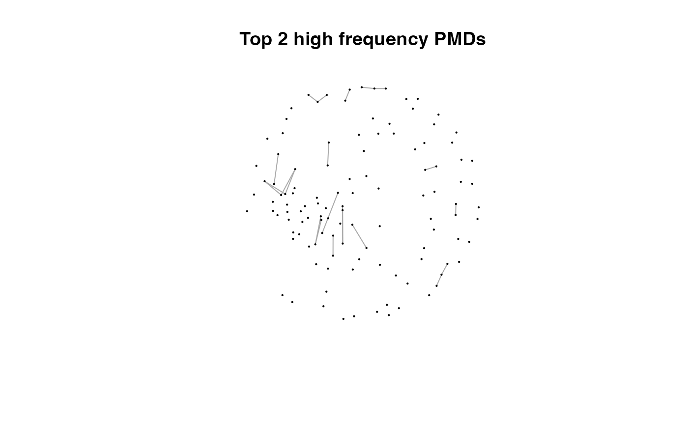
Here we could find more and more compounds will be connected with more high frequency PMDs. Meanwhile, the mean distance of all network nodes will increase. However, some PMDs are generated by random combination of ions. In this case, if we included those PMDs for the network, the mean distance of all network nodes will decrease. Here, the largest mean distance means no more information will be found for certain data set and such value is used as the cutoff for high frequency PMDs selection.

You could use plotstdsda to show the distribution of the selected paired peaks.

plotstdsda(sda)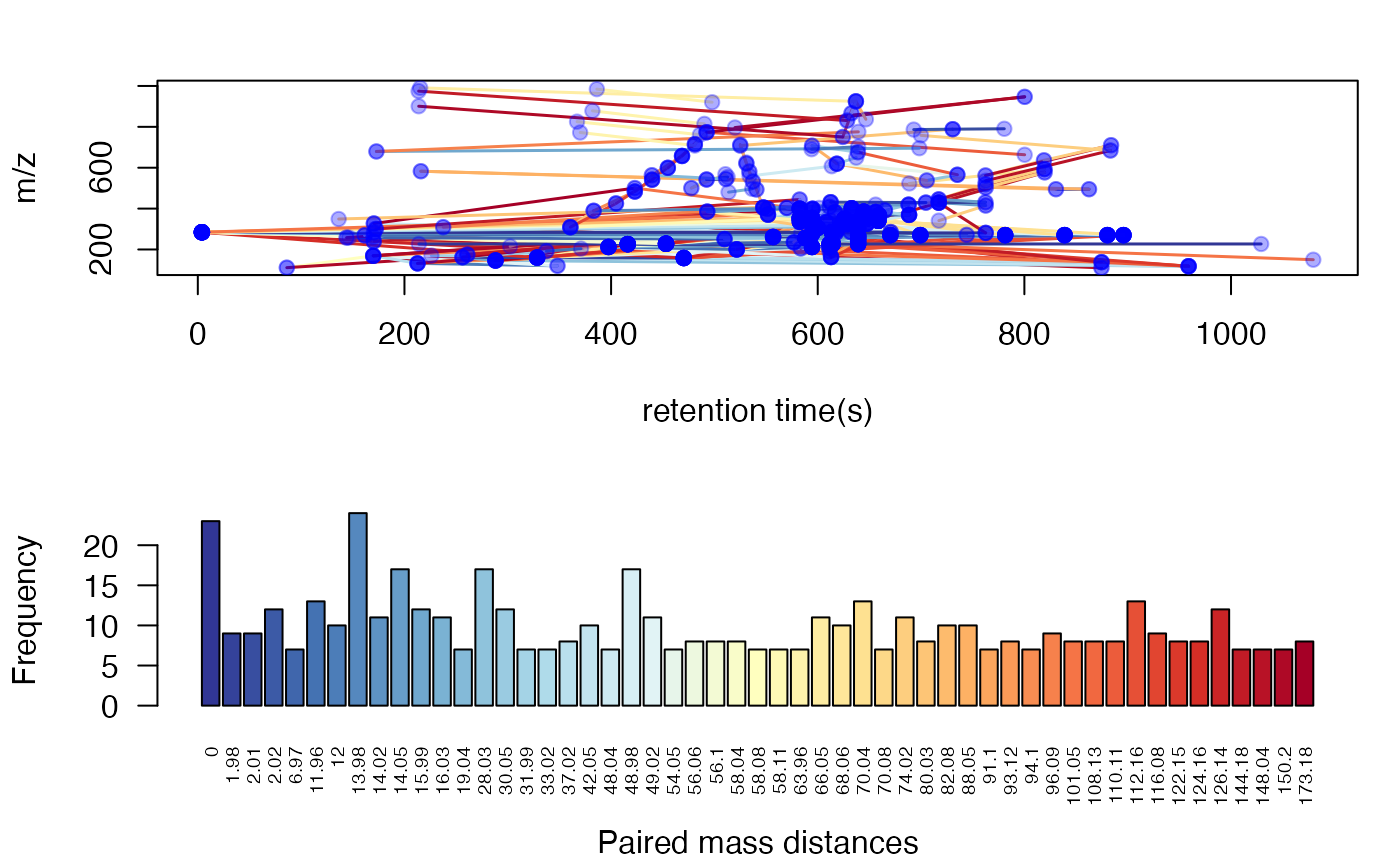

You could also use index to show the distribution of certain PMDs.

par(mfrow = c(1,3),mar = c(4,4,2,1)+0.1)
plotstdsda(sda,sda$sda$diff2 == 2.02)
plotstdsda(sda,sda$sda$diff2 == 28.03)
plotstdsda(sda,sda$sda$diff2 == 58.04)

Structure/reaction directed analysis could be directly performed on all the peaks, which is slow to process:

sdaall <- getsda(spmeinvivo)
#> PMD frequency cutoff is 104 by PMD network analysis with largest network average distance 14.06 .
#> 6 groups were found as high frequency PMD group.
#> 0 was found as high frequency PMD. 
#> 2.02 was found as high frequency PMD. 
#> 28.03 was found as high frequency PMD. 
#> 31.01 was found as high frequency PMD. 
#> 58.04 was found as high frequency PMD. 
#> 116.08 was found as high frequency PMD.

par(mfrow = c(1,3),mar = c(4,4,2,1)+0.1)
plotstdsda(sdaall,sdaall$sda$diff2 == 2.02)
plotstdsda(sdaall,sdaall$sda$diff2 == 28.03)
plotstdsda(sdaall,sdaall$sda$diff2 == 58.04)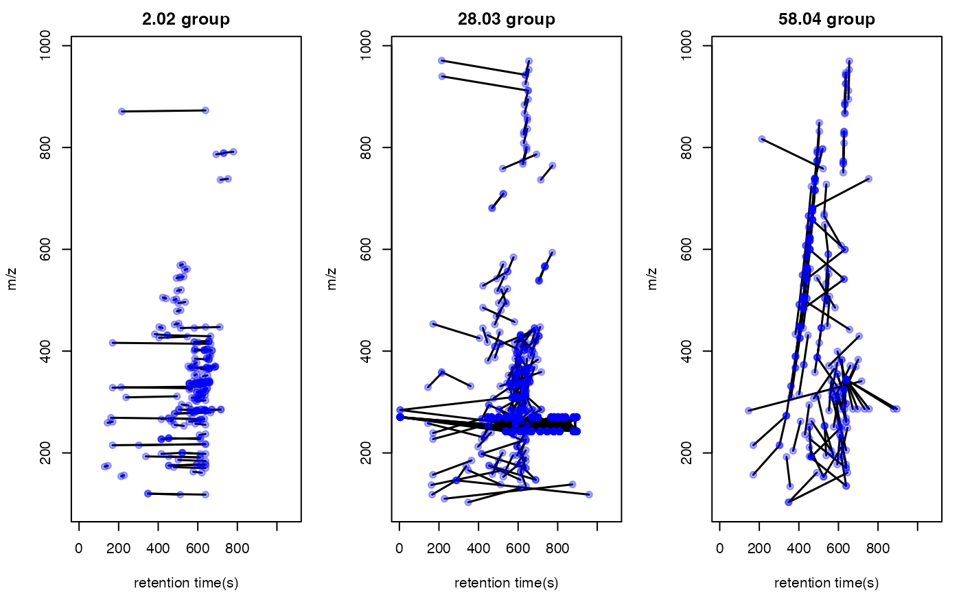

Extra filter with correlation coefficient cutoff

Structure/Reaction directed analysis could also use correlation to restrict the paired ions. However, similar to GlobalStd algorithm, such cutoff will remove low intensity data. Researcher should have a clear idea to use this cutoff.

sda2 <- getsda(std, corcutoff = 0.9)
#> PMD frequency cutoff is 6 by PMD network analysis with largest network average distance 6.67 .
#> 41 groups were found as high frequency PMD group.
#> 0 was found as high frequency PMD. 
#> 1.98 was found as high frequency PMD. 
#> 2.01 was found as high frequency PMD. 
#> 2.02 was found as high frequency PMD. 
#> 11.96 was found as high frequency PMD. 
#> 12 was found as high frequency PMD. 
#> 13.98 was found as high frequency PMD. 
#> 14.02 was found as high frequency PMD. 
#> 14.05 was found as high frequency PMD. 
#> 15.99 was found as high frequency PMD. 
#> 16.03 was found as high frequency PMD. 
#> 19.04 was found as high frequency PMD. 
#> 28.03 was found as high frequency PMD. 
#> 30.05 was found as high frequency PMD. 
#> 31.99 was found as high frequency PMD. 
#> 33.02 was found as high frequency PMD. 
#> 42.05 was found as high frequency PMD. 
#> 48.98 was found as high frequency PMD. 
#> 49.02 was found as high frequency PMD. 
#> 54.05 was found as high frequency PMD. 
#> 56.06 was found as high frequency PMD. 
#> 58.04 was found as high frequency PMD. 
#> 58.08 was found as high frequency PMD. 
#> 63.96 was found as high frequency PMD. 
#> 66.05 was found as high frequency PMD. 
#> 68.06 was found as high frequency PMD. 
#> 70.08 was found as high frequency PMD. 
#> 74.02 was found as high frequency PMD. 
#> 80.03 was found as high frequency PMD. 
#> 82.08 was found as high frequency PMD. 
#> 88.05 was found as high frequency PMD. 
#> 93.12 was found as high frequency PMD. 
#> 94.1 was found as high frequency PMD. 
#> 96.09 was found as high frequency PMD. 
#> 108.13 was found as high frequency PMD. 
#> 110.11 was found as high frequency PMD. 
#> 112.16 was found as high frequency PMD. 
#> 116.08 was found as high frequency PMD. 
#> 122.15 was found as high frequency PMD. 
#> 124.16 was found as high frequency PMD. 
#> 126.14 was found as high frequency PMD.

plotstdsda(sda2)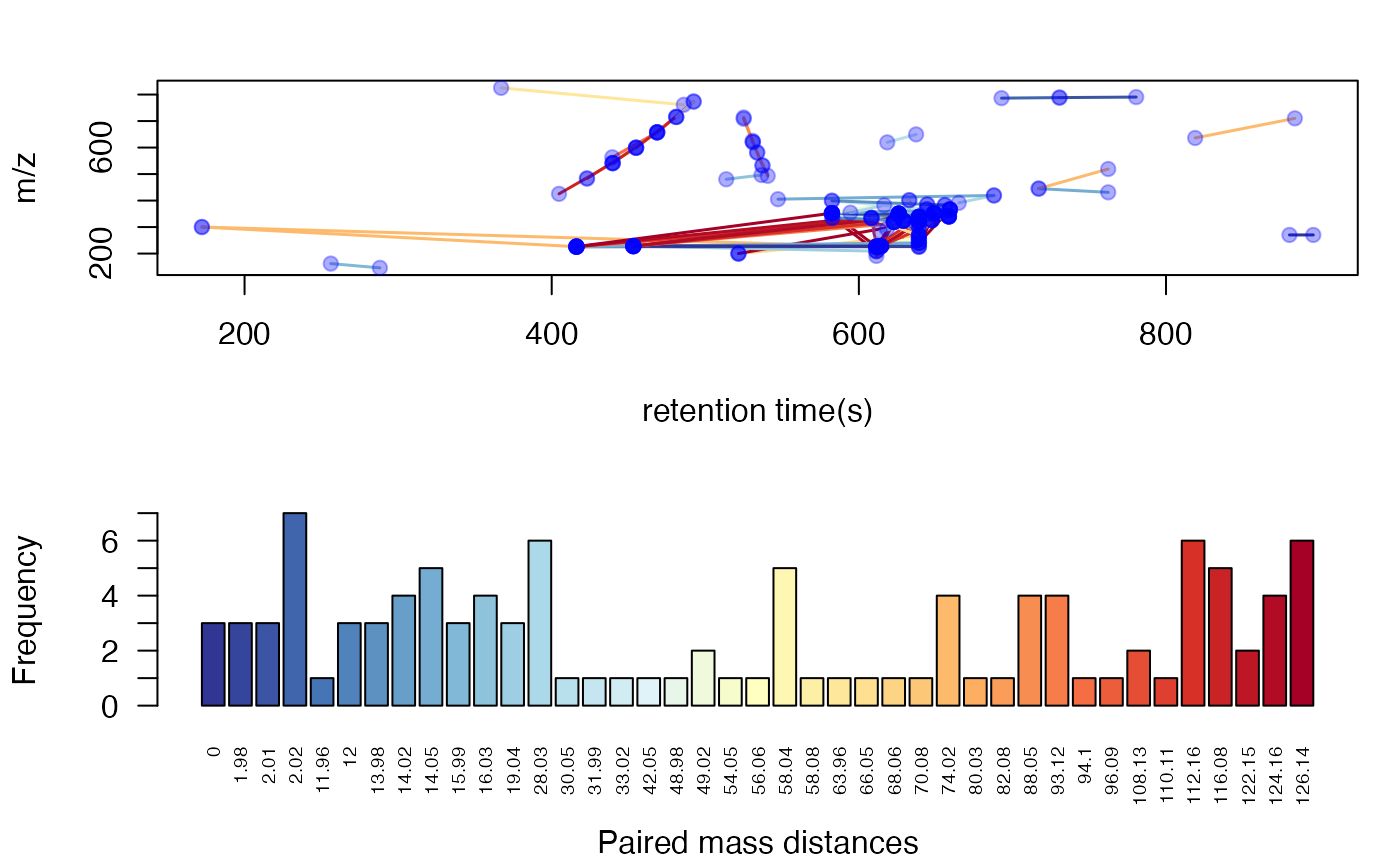

Structure/reaction directed analysis for peaks/compounds only data

When you only have data of peaks without retention time or compounds list, structure/reaction directed analysis could also be done by getrda function.

sda <- getrda(spmeinvivo$mz)
#> 164462 pmd found.
#> 20 pmd used.

# check high frequency pmd
colnames(sda)
#>  [1] "0"       "1.001"   "1.002"   "1.003"   "1.004"   "2.015"   "2.016"  
#>  [8] "14.015"  "17.026"  "18.011"  "21.982"  "28.031"  "28.032"  "44.026" 
#> [15] "67.987"  "67.988"  "88.052"  "116.192" "135.974" "135.975"

# get certain pmd related m/z
idx <- sda[,'2.016']
# show the m/z
spmeinvivo$mz[idx]
#>  [1] 118.0651 118.0652 120.0812 159.1575 162.0552 170.0330 170.0932 170.1541
#>  [9] 174.1363 174.9917 175.0873 176.0305 176.0418 181.9872 184.1695 188.6484
#> [17] 192.1487 192.1604 226.9522 226.9523 228.1969 228.1973 259.1148 261.1317
#> [25] 270.3185 271.3217 272.3230 272.3234 273.8902 274.8744 284.2955 285.3002
#> [33] 285.3002 286.3101 286.3101 291.0712 293.1755 294.9392 296.2961 304.3081
#> [41] 305.2480 305.3118 308.0889 308.2953 308.2954 309.1672 309.2046 315.1781
#> [49] 317.9344 319.3005 319.3002 319.9302 320.3041 320.3322 321.3165 322.3185
#> [57] 323.3221 324.3266 325.3294 327.2022 327.3449 329.0052 331.0031 350.3426
#> [65] 352.3214 352.3215 353.3244 354.3365 355.0696 359.2410 361.2353 372.3197
#> [73] 375.3066 383.2804 383.3723 384.3350 385.2753 385.3480 387.2851 397.1907
#> [81] 399.3274 400.9174 401.3420 403.2859 432.8860 433.2781 445.8289 447.1173
#> [89] 451.3633 462.8615 522.3557 524.1178 525.9831 526.4841 705.7223 708.8218
#> [97] 976.3139 976.8122 982.7763

Wrap function for GlobalStd algorithm

globalstd function is a wrap function to process GlobalStd algorithm and structure/reaction directed analysis in one line. All the plot function could be directly used on the list objects from globalstd function. If you want to perform structure/reaction directed analysis, set the sda=T in the globalstd function.

result <- globalstd(spmeinvivo, sda=FALSE)
#> 75 retention time cluster found.
#> 369 paired masses found
#> 5 unique within RT clusters high frequency PMD(s) used for further investigation.
#> The unique within RT clusters high frequency PMD(s) is(are)  28.03 21.98 44.03 17.03 18.01.
#> 719 isotopologue(s) related paired mass found.
#> 492 multi-charger(s) related paired mass found.
#> 8 retention group(s) have single peaks. 14 23 32 33 54 55 56 75
#> 11 group(s) with multiple peaks while no isotope/paired relationship 4 5 7 8 11 41 42 49 68 72 73
#> 9 group(s) with multiple peaks with isotope without paired relationship 2 9 22 26 52 62 64 66 70
#> 4 group(s) with paired relationship without isotope 1 10 15 18
#> 43 group(s) with paired relationship and isotope 3 6 12 13 16 17 19 20 21 24 25 27 28 29 30 31 34 35 36 37 38 39 40 43 44 45 46 47 48 50 51 53 57 58 59 60 61 63 65 67 69 71 74
#> 291 std mass found.

Use independent peaks for MS/MS validation (PMDDA)

Independent peaks are supposing generated from different compounds. We could use those peaks for MS/MS analysis instead of DIA or DDA. Here we need multiple injections for one sample since it might be impossible to get all ions’ fragment ions in one injection with good sensitivity. You could use gettarget to generate the index for the injections and output the peaks for each run.

# you need retention time for independent peaks
index <- gettarget(std$rt[std$stdmassindex])
#> You need 10 injections!

# output the ions for each injection
table(index)
#> index
#>  1  2  3  4  5  6  7  8  9 10 
#> 25 28 40 18 28 29 34 45 28 16

# show the ions for the first injection
std$mz[index==1]
#>   [1] 110.0717 114.0918 122.9247 125.9874 133.0794 137.9879 141.9594 149.9530
#>   [9] 165.0787 166.0867 172.1705 174.9383 175.1482 183.0809 193.1599 198.1854
#>  [17] 203.0532 205.0872 205.1954 220.1184 226.1823 242.2863 242.9260 255.2511
#>  [25] 259.9651 264.1944 267.0639 270.3185 270.3172 270.3185 270.3184 271.3216
#>  [33] 273.8902 285.3002 286.3101 294.2054 296.9066 300.2046 306.2514 310.3117
#>  [41] 315.1781 317.9344 319.3005 319.9302 329.8840 334.3101 349.3476 351.3455
#>  [49] 363.3114 367.2694 371.3345 374.3041 380.0033 382.3673 383.2804 386.3523
#>  [57] 391.2835 394.8754 410.2585 411.0941 417.2462 420.3193 424.0815 430.0895
#>  [65] 437.2355 445.2767 445.3874 446.8878 447.2935 467.1031 471.3317 505.1055
#>  [73] 507.3303 527.2976 536.1655 540.8890 542.3991 548.2764 551.3562 556.8633
#>  [81] 560.3877 564.1885 567.1783 586.4524 589.5800 600.4401 605.2231 608.4285
#>  [89] 620.4358 636.1983 643.4632 646.4585 649.6613 650.8519 669.4185 675.5084
#>  [97] 703.3651 704.1390 720.8364 732.5472 739.6479 750.6089 758.4735 760.8210
#> [105] 764.8339 771.8544 773.6523 779.5153 803.5434 804.8442 816.5102 826.6806
#> [113] 832.8212 840.8392 861.5014 870.7857 872.3052 872.8314 873.3343 889.8086
#> [121] 900.3092 942.7638 946.7164 979.7901 991.7894

std$rt[index==1]
#>   [1]  228.0840  172.8550  217.9690 1079.6500  212.6560  165.4680 1079.4300
#>   [8] 1079.6400  511.3690  348.1340  478.9360  216.1500  453.1780  533.7950
#>  [15]  453.1780  415.9985  144.8840  583.5530  639.1010  170.8240  611.4120
#>  [22]  780.5760  216.0600  639.1000  145.9660  473.1445  568.7680  538.0815
#>  [29]    4.0610  604.7690  465.0070  781.0040  145.9680  716.7800  631.8770
#>  [36]  452.0005  145.1090  172.2230  599.6270  618.4820  401.2135  145.5170
#>  [43]  622.7690  145.2280  144.3380  608.1990  659.2440  626.0920  561.2685
#>  [50]  382.6770  551.7325  582.4840  212.9175  616.5550  547.0180  644.4580
#>  [57]  665.0280  217.1550  633.9130  563.1970  444.6075  687.8085  583.9830
#>  [64]  717.1010  170.9435  421.8915  582.4825  215.6320  404.5340  717.1030
#>  [71]  540.8660  762.4675  554.8390  493.5080  762.5770  213.7260  439.6780
#>  [78]  493.5080  551.4100  215.9830  533.3660  762.5770  762.3630  439.2500
#>  [85]  889.0520  455.1500  762.5750  613.3395  531.0080  818.9800  449.3200
#>  [92]  605.8410  637.2775  215.6410  527.7950  468.2215  213.5480  639.1000
#>  [99]  215.1360  481.0785  639.1005  624.2710  522.4370  215.6320  213.7270
#> [106]  213.7720  613.5550  519.6690  665.0290  213.5090  213.3340  628.4480
#> [113]  213.7130  213.9270  213.3395  216.5120  639.0990  213.5090  213.5480
#> [120]  215.2605  213.5480  636.9060  637.1710  213.9410  215.3500

Shiny application

An interactive document has been included in this package to perform PMD analysis. You need to prepare a csv file with m/z and retention time of peaks. Such csv file could be generated by run enviGCMS::getcsv() on the list object from enviGCMS::getmzrt(xset) function. The xset should be XCMSnExp object or xcmsSet object. You could also generate the csv file by enviGCMS::getmzrt(xset,name = 'test'). You will find the csv file in the working dictionary named test.csv.

Then you could run runPMD() to start the Graphical user interface(GUI) for GlobalStd algorithm and structure/reaction directed analysis.

Conclusion

pmd package could be used to reduce the redundancy peaks for GC/LC-MS based research and perform structure/reaction directed analysis to screen known and unknown important compounds or reactions.

Miao Yu

2024-05-30

Introduction of Paired Mass Distance analysis

PMD from the same compound

PMD from different compounds

Data format

GlobalStd algorithm

STEP1: Retention time hierarchical clustering

STEP2: Relationship among adducts, neutral loss, isotopologues and common fragments ions

STEP3: Screen the independent peaks

Extra filter with correlation coefficient cutoff

Validation by principal components analysis(PCA)

Comparison with other pseudo spectra extraction method

Structure/Reaction directed analysis

Extra filter with correlation coefficient cutoff

Structure/reaction directed analysis for peaks/compounds only data

Wrap function for GlobalStd algorithm

Use independent peaks for MS/MS validation (PMDDA)

Shiny application

Conclusion